1. Introduction

The accuracy of temperature forecasts is crucial for the global response to climate change and for developing corresponding decisions. Climate change has a huge impact on agriculture, which is increasingly at risk due to its heightened sensitivity and vulnerability to climate change [1-3]. And Climate change has emerged as the most rapidly increasing global threat to human well-being [4]. Accurate forecasts can better assist governments and organizations in developing effective strategies to mitigate the impact of climate change on both nature and humans, providing a scientific basis for addressing extreme weather events.

How to accurately predict global temperature anomalies through data modeling is still a key topic in climate change research. Early climate prediction research mainly relied on physical models, but with the continuous development of statistical methods, traditional time series models such as ARIMA have been gradually applied in climate prediction. These models can effectively capture the long-term characteristics of climate change by analyzing trends and fluctuations in historical data [5-7]. For example, ARIMA models perform well in the prediction of variables such as global temperature and precipitation and provide more accurate results especially when dealing with long-term and stable time series [8-10]. With reliable predictions of future temperature changes, governments and related organizations can develop more effective countermeasures to help reduce the potential impacts of climate change on human life and ecosystems. Therefore, accurate temperature prediction is not only important in academic research but also provides a scientific basis for climate risk management in reality.

In this paper, based on the global temperature anomaly data provided by NASA GISTEMP from 1880 to the present, ARIMA and ETS models are used for modeling and prediction respectively. The main tasks of the study include preprocessing and time series transformation of the global temperature anomaly data, model fitting in ARIMA and ETS models, comparing the forecasting effects of the two models, and validating the models through residual analysis and error assessment. By evaluating the performance of these two traditional time series models, this paper aims to provide a reference basis for long-term global temperature prediction and to find a new direction for future climate change research.

2. Data and Methods

2.1. Data

This study uses data from NASA GISTEMP global temperature anomalies from 1880 to the present. The data records temperature outliers on a global scale on a monthly basis. By loading and cleaning the data, removing missing values, and converting them into a time series format, subsequent modeling ensures that long-term trends in global temperatures are better captured. Figure 1 shows the trend of global temperature anomalies from 1880 to the present. As can be seen from the figure, the global temperature has gradually increased since the 20th century, especially the temperature anomaly in the early 21st century, reflecting the intensified trend of climate change.

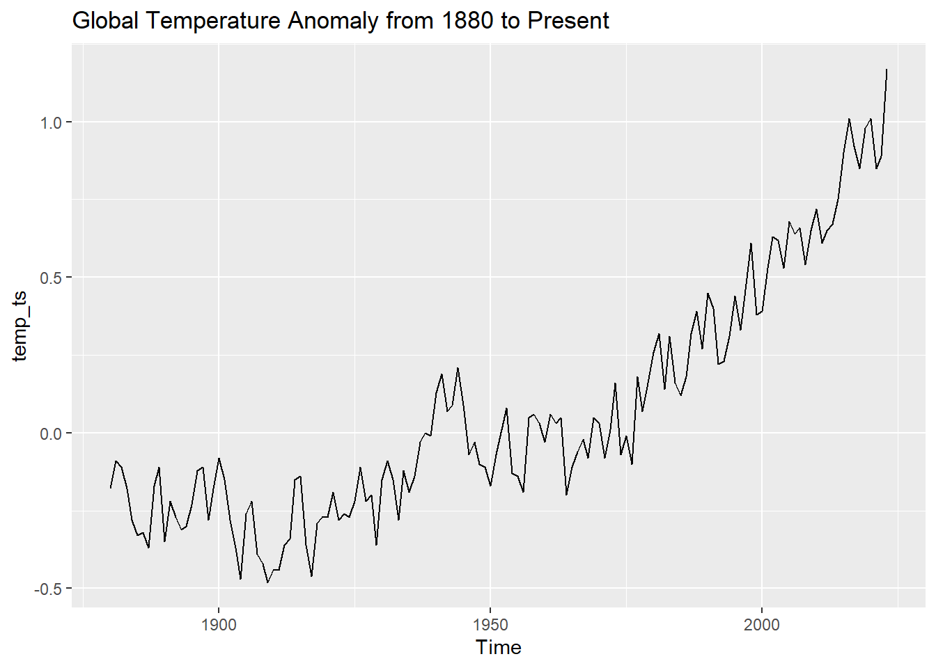
Figure 1: Global Temperature Anomaly from 1880 to present

Subsequently, to better observe the long-term trend of global temperature anomalies, the five-year moving average data was smoothed. To smooth out short-term volatility and highlight changing trends.

2.2. Dataset Division

To evaluate the model's predictive performance, the dataset is split into a training set and a test set. The training set, consisting of data from 1880 to 1980, is used to train the model, while the test set, containing data from 1981 to the present, is utilized for model validation and testing. This approach is an effective way to assess the model's ability to predict future temperature trends, particularly when working with long-term data.

2.3. ARIMA Model

The ARIMA model is suitable for handling non-stationary time series data, as it transforms non-stationary series into stationary ones through differencing operations. The global temperature anomaly data exhibit significant trend changes and their statistical properties are not stable over time. The ARIMA model predicts future changes by differing the series to achieve stationarity, followed by applying autoregressive and moving average components. ARIMA models can be used to confirm both regional and global warming through their predictive capabilities [11]. This makes it well-suited for long-term temperature forecasting, particularly when significant seasonal effects are absent. The ARIMA model primarily consists of three components. First, autoregressive (AR) represents the correlation between the current data point and the previous data points. Second, differencing (I) is used to transform non-stationary sequences into stationary ones. Finally, the moving average (MA) component reflects the correlation between the current data point and the previous few residuals. Through these three components, the ARIMA model can effectively capture the trend and random fluctuations of time series. The complete form of an ARIMA model is shown as follows in Equation (1).

In formula. lag operator is denoted by L, autoregressive coefficient is denoted by ϕi, moving average coefficient is denoted by θi, order of differencing is d, and ϵt is the white noise error term. Over the difference operation (1 - L) d, the non-smooth time series can be transformed into a smooth series, while the autoregressive and moving average parts predict the future values through the lagged values and error terms.

2.4. ETS Model

The ETS model is particularly suitable for time series with distinct trends and seasonal patterns. By breaking the data down into error, trend, and seasonal components, it efficiently captures both long-term changes and cyclical fluctuations, offering potential advantages in identifying trends. The flexibility of the ETS model lies in its ability to accommodate trend and seasonal components with different characteristics, describe these changes by addition or multiplication, and is suitable for time series forecasting with trend characteristics [12]. The ETS model works by decomposing the time series into three key components. First, the error (E), which accounts for the unpredictable random variations in the time series. Second, the trend (T), representing the long-term direction or movement of the data. Finally, the seasonality (S), which captures the cyclical fluctuations within the data. The ETS model is usually denoted in its specific form by three letters corresponding to the error, trend, and seasonality components. In this case, the model is ETS (A, N, N), i.e. additive error, no trend, and no seasonality. The model assumes that changes in temperature anomaly data are mainly controlled by additive errors and is suitable for capturing long-term trends in global temperatures. Thus obtain the full form of the ETS model as follows in Equation (2).

The ETS model is applicable to time series with significant trends and seasonal components. The ETS model is effective in capturing long-term changes and cyclical fluctuations in the data by decomposing the data into error, trend, and seasonal components. The ETS model is effective in capturing the trend in which the predicted value of Yt time t. The level of ℓt time t denotes the smooth baseline value. bt time t of trend, denotes the long-term change in the data. st time t of seasonal, denotes cyclical fluctuations in the data. ϵt error into, denotes random fluctuations. trend. st seasons at time t, denoting cyclical fluctuations. The ETS model is especially well-suited to time series that exhibit clear trends and seasonal patterns. By breaking the data down into error, trend, and seasonal components, it efficiently captures both long-term changes and cyclical fluctuations. The ETS model is well-suited for time series that exhibit pronounced trends and seasonal patterns. By decomposing the data into error, trend, and seasonal components, the model effectively captures long-term shifts and cyclical variationsations in the data. ϵt errors into, denoting stochastic fluctuations. In the chosen ETS (A, N, N) model, the trend and seasonal components are ignored i.e., bt and st are absent.

3. Results

3.1. Model Fitting Results

ARIMA and ETS models were fitted using NASA GISTEM data from 1880 to 1980 as a training model and data from 1981 to the present as a test set. The ARIMA and ETS models were each fitted using the training set data. The ARIMA model, with an AIC value of -170.38 and a BIC value of -157.35, demonstrates a better fit. In contrast, the ETS model has an AIC value of 14.94504 and a BIC value of 22.79040, indicating a slightly poorer fit compared to the ARIMA model.

3.2. Visualization of Forecasting Results

Figure 2 shows the actual data (red line) of the global temperature anomaly and the prediction results based on the ARIMA and ETS models. It can be seen that the fitting results of the ARIMA model (green line) are closer to the actual data, while the prediction results of the ETS model (blue line) deviate from the actual data, showing that the fitting is not as effective as the ARIMA model.

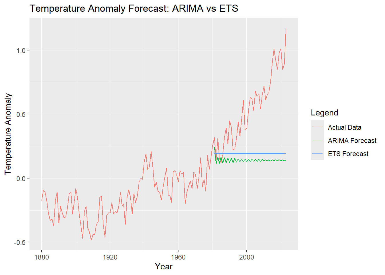
Figure 2: Temperature Anomaly Forecast: ARIMA vs ETS

3.3. Residual Analysis

The results of the residual analysis for the ARIMA (1,1,3) model are presented in Figure 3, demonstrating no significant autocorrelation in the residuals. The p-value of the Ljung-Box test is 0.9992, indicating that the residuals follow white noise, and the model has a good fitting effect. Similarly, Figure 4 displays the residual analysis for the ETS (A, N, N) model, where the p-value of the Ljung-Box test is 0.4753, showing no significant autocorrelation in the residuals. However, the fitting effect of the ETS model is inferior to that of the ARIMA model.

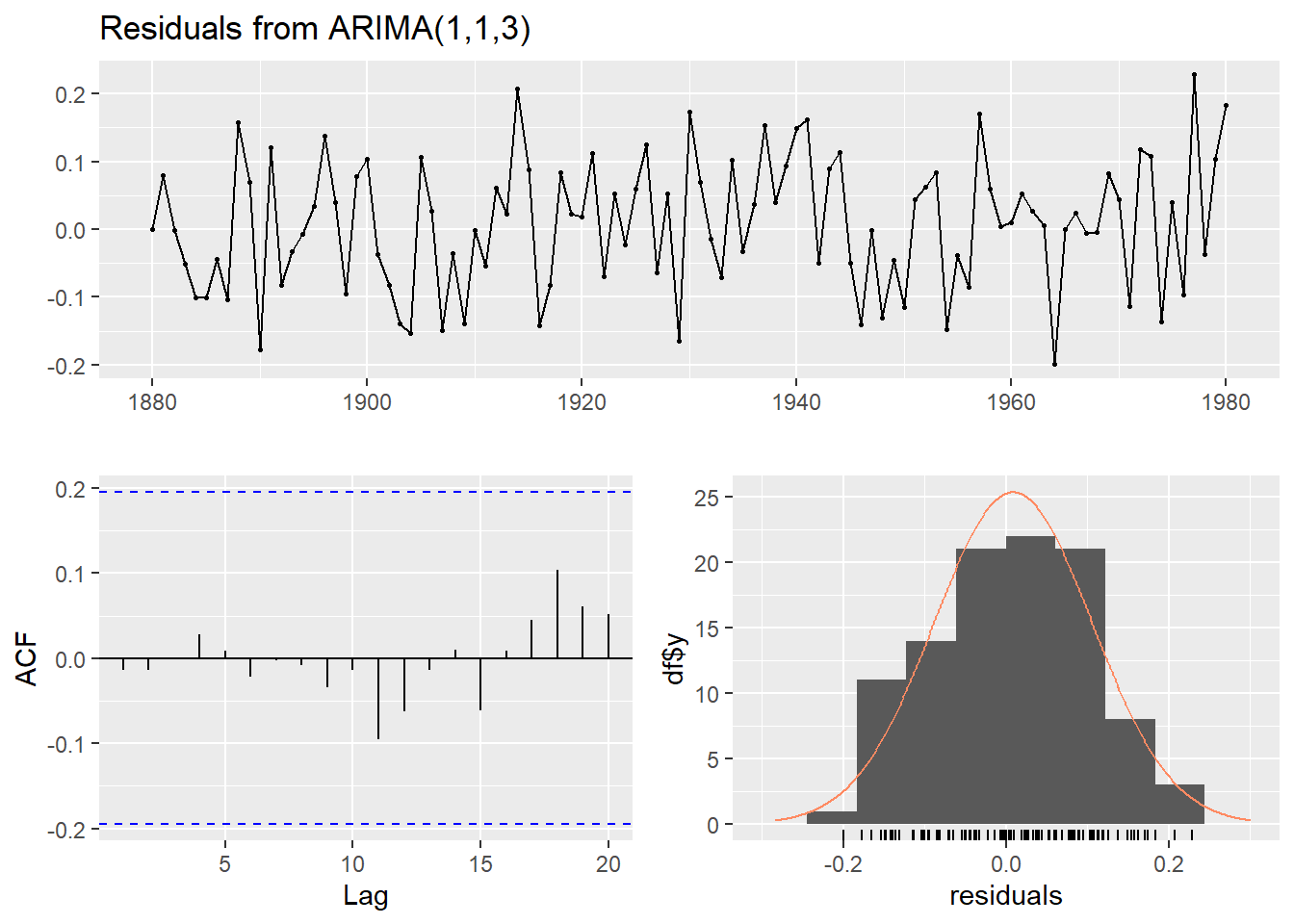
Figure 3: Residuals from ARIMA (1,1,3)

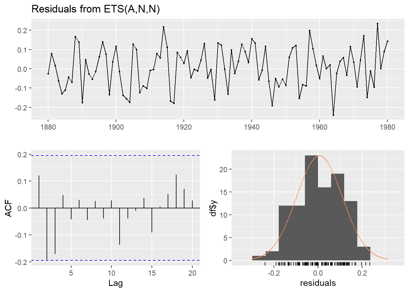
Figure 4: Residuals from ETS

3.4. Model Performance Evaluation

To comprehensively assess the predictive ability of the ARIMA and ETS models, the evaluation will be based on indicators such as MSE, AIC, and BIC to compare the forecasting performance of both models. As can be seen in Table 1, the ARIMA model has a slightly higher MSE value (0.2428396) compared to the ETS model (0.2024324), It indicates that the ARIMA model has a slight disadvantage in this indicator. However, the AIC (-170.3803) and BIC (-157.35) of the ARIMA model's values are significantly lower compared to those of the ETS model, indicating that the ARIMA model has a better performance in terms of model complexity and residual processing. In addition to this, the Ljung-Box test p-value of ARIMA is 0.9992, while the ETS model has a p-value of 0.4753, indicating that its residual autocorrelation is stronger, which may capture some of the noise. Although the MSE of the ETS model is slightly lower, considering the results together, the ARIMA model performs superior in dealing with long-term trend forecasting. The ETS model is more suitable for short-term forecasting, while the ARIMA model is more suitable for long-term forecasting of global anomaly data.

Table 1: The evaluation metrics for ARIMA and ETS models

4. Conclusion

In this study, by analyzing the global temperature anomaly data from NASA GISTEMP 1880 to the present, projections of global temperature anomalies were made using ARIMA and ETS models separately. The analysis and comparison show that ARIMA performs better than ETS in long-term forecasts, especially in dealing with time series without obvious seasonal components. The ETS model has a lower error when dealing with more volatile data, and although the ETS model has a slight advantage in MSE, the ETS model does not perform as well as the ARIMA model in long-term forecasting when considering AIC, BIC, and other indicators.

Future research could incorporate more advanced forecasting models, such as machine learning or hybrid models. In addition, further research can be conducted on how to combine different data sources to enhance the predictive ability of the model. Meanwhile, more external influences, such as carbon dioxide concentration, can be considered to improve the accuracy of temperature anomaly predictions and provide a more reliable basis for temperature changes.

References

[1]. Dong, Z., Pan, Z., An, P., et al. (2018). A quantitative method for risk assessment of agriculture due to climate change. 131(1-2), 653–659.
[2]. Kar, S. K., Sharma, A., Kar, S., & Dey, A. (2024). Impact on Agricultural Crop Production Under Climate Change Scenario. Springer EBooks, 109–132.
[3]. Thottadi, B. P., & Singh, S. P. (2024). Climate-smart agriculture (CSA) adaptation, adaptation determinants and extension services synergies: a systematic review. Mitigation and Adaptation Strategies for Global Change, 29(3).
[4]. Shivanna, K. R. (2022). Climate change and its impact on biodiversity and human welfare. DELETED, 88(2), 160–171.
[5]. Jain, G., & Mallick, B. (2017). A study of time series models ARIMA and ETS. Available at SSRN 2898968.
[6]. Wang, H., Huang, J., Zhou, H., Zhao, L., & Yuan, Y. (2019). An integrated variational mode decomposition and ARIMA model to forecast air temperature. Sustainability, 11(15), 4018.
[7]. Dimri, T., Ahmad, S., & Sharif, M. (2020). Time series analysis of climate variables using seasonal ARIMA approach. Journal of Earth System Science, 129(1).
[8]. Lai, Y., & Dzombak, D. A. (2020). Use of the Autoregressive Integrated Moving Average (ARIMA) model to forecast Near-Term regional temperature and precipitation. Weather and Forecasting, 35(3), 959–976.
[9]. Xu, D., Zhang, Q., Ding, Y., & Zhang, D. (2021). Application of a hybrid ARIMA-LSTM model based on the SPEI for drought forecasting. Environmental Science and Pollution Research, 29(3), 4128–4144.
[10]. Machekposhti, K. H., Sedghi, H., Telvari, A., & Babazadeh, H. (2018). Modeling Climate Variables of Rivers Basin using Time Series Analysis (Case Study: Karkheh River Basin at Iran). Civil Engineering Journal, 4(1), 78.
[11]. Amjad, M., Khan, A., Fatima, K., Ajaz, O., Ali, S., & Main, K. (2022). Analysis of temperature variability, trends and prediction in the Karachi region of Pakistan using ARIMA models. Atmosphere, 14(1), 88.
[12]. Jofipasi, C. A., Miftahuddin, N., & Hizir, N. (2018). Selection for the best ETS (error, trend, seasonal) model to forecast weather in the Aceh Besar District. IOP Conference Series Materials Science and Engineering, 352, 012055.
Cite this article
Fan,C. (2025). Global Temperature Anomaly Forecast: A Comparative Analysis of ARIMA and ETS Models. Advances in Economics, Management and Political Sciences,144,70-76.
Data availability
The datasets used and/or analyzed during the current study will be available from the authors upon reasonable request.
Disclaimer/Publisher's Note
The statements, opinions and data contained in all publications are solely those of the individual author(s) and contributor(s) and not of EWA Publishing and/or the editor(s). EWA Publishing and/or the editor(s) disclaim responsibility for any injury to people or property resulting from any ideas, methods, instructions or products referred to in the content.
About volume
Volume title: Proceedings of ICFTBA 2024 Workshop: Finance's Role in the Just Transition
© 2024 by the author(s). Licensee EWA Publishing, Oxford, UK. This article is an open access article distributed under the terms and
conditions of the Creative Commons Attribution (CC BY) license. Authors who
publish this series agree to the following terms:
1. Authors retain copyright and grant the series right of first publication with the work simultaneously licensed under a Creative Commons
Attribution License that allows others to share the work with an acknowledgment of the work's authorship and initial publication in this
series.
2. Authors are able to enter into separate, additional contractual arrangements for the non-exclusive distribution of the series's published
version of the work (e.g., post it to an institutional repository or publish it in a book), with an acknowledgment of its initial
publication in this series.
3. Authors are permitted and encouraged to post their work online (e.g., in institutional repositories or on their website) prior to and
during the submission process, as it can lead to productive exchanges, as well as earlier and greater citation of published work (See
Open access policy for details).