1. Introduction

The Nikkei 225 is the most representative index of the Japanese stock market, consisting of 225 stocks picked from those listed on the Tokyo Stock Exchange using the price averaging method. As such, it not only reflects the general performance of the Japanese stock market, but it additionally has an unbreakable connection to the global economy. Studies show that the Nikkei's volatility is driven not only by domestic economic problems but also by global markets and international macroeconomic policies [1]. Furthermore, according to the research by Beltratti and Morana, the Nikkei 225's volatility is influenced by global macroeconomic policies and international stock market fluctuations, illustrating its powerful correlation with the global financial system[2]. Given the Nikkei's extreme volatility and complexity, precisely anticipating its movement is crucial for investors and economic authorities. Meanwhile, the ARIMA model is increasingly widespread in financial markets for short-term forecasting due to its effectiveness in time series analysis. Besides, Box and Jenkins emphasized that the ARIMA model can forecast volatile data such as the Nikkei through investigating the auto-correlation and trend of the time series, and it is particularly successful for forecasting short-term trends in non-stationary data.

The Nikkei 225 Index is forecasted and analyzed using the ARIMA(1,1,0) model from September 2022 to September 2024. The results demonstrate the model's high short-term prediction accuracy, particularly with regard to the market's performance over the next 30 days, which exhibits a more stable trend consistent with the short-term stabilizing characteristics of the stock market. Nevertheless, as the prediction period lengthens, the model's confidence interval steadily widens and the prediction's uncertainty develops, this is especially noticeable when the market varies dramatically, thereby lowering the model's accuracy. During the research procedure, the data were preprocessed, smoothness tested, and inspected for missing or outlier data. Following that, the ARIMA model was built, and the best model was determined using the AIC and BIC criteria. It is discovered that while the ARIMA model has certain limitations in long-term complicated unstable markets, it is appropriate for short-term forecasting. Last but not least, this article suggests that future developments in the manner of exogenous variable inclusion like macroeconomic policies or the adoption of more complicated models such as GARCH could enhance the model's accuracy in long-term forecasting.

2. Data

Initially, it is necessary to verify and preprocess the data.

2.1. Data source

The historical data for Nikkei225 from Sep 2022 to Sep 2024 are downloaded from https://finance.yahoo.com/. The relevant indicators include date, open price, close price, high price, low price, and volume. Besides, through analyzing the structure of these variables, except date is a categorical variable, all other variables are continuous variables capable of reflecting the changing trend of the data over a certain period. In stock market analysis, variables like open, high, low, and volume provide key insights into market behavior. However, the closing price is an essential forecasting element since it reflects the market’s final sentiment [3].

2.2. Data Processing

2.2.1. Data Check

According to Figure 1, the majority of closing prices ranged between 25,000 and 40,000. Furthermore, the data contains no missing values, with each column having a missing value count of 0. There are no missing values or outliers in the Nikkei index data, consequently no additional data preprocessing is necessary.

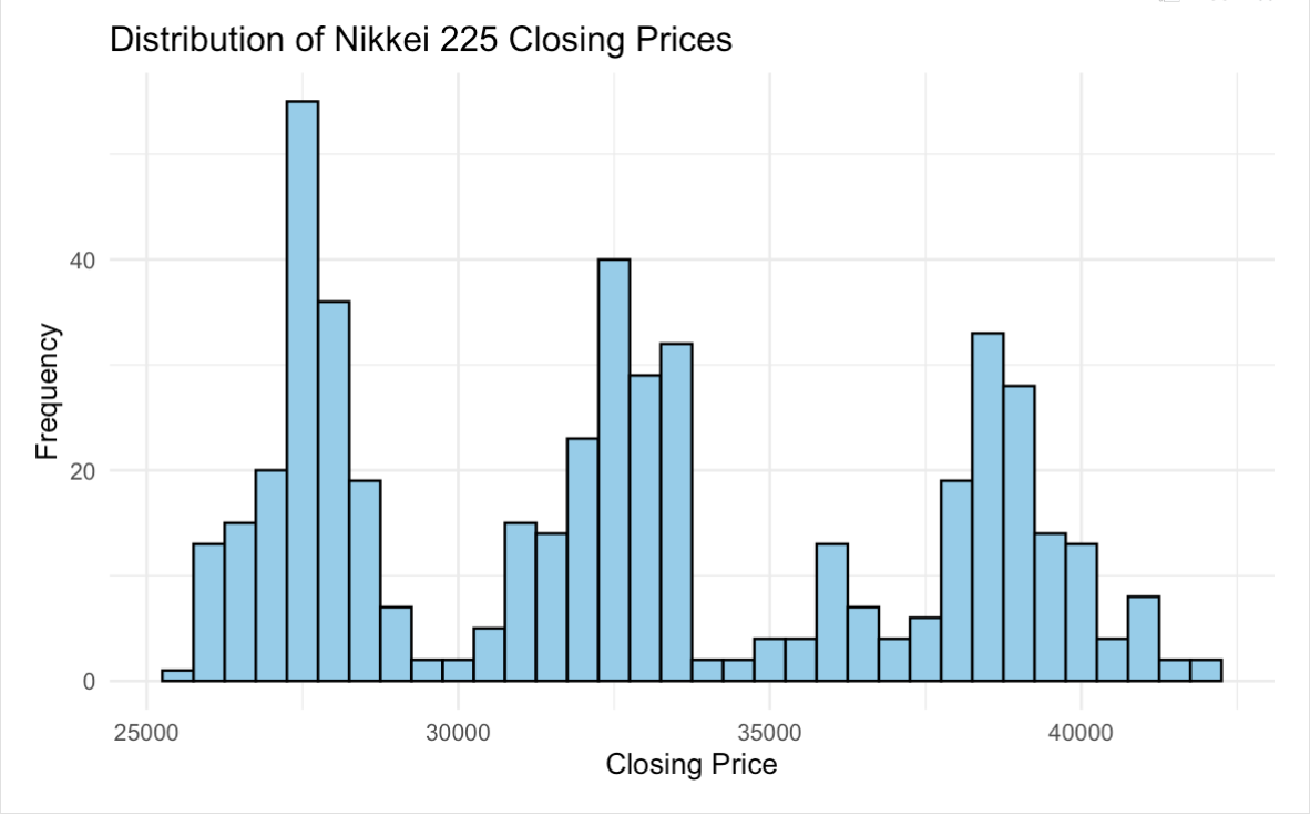
Figure 1: Distribution of Nikkei 225 Closing Prices (Picture Credit: Original)

2.2.2. Stationary test

Because non-stationary series might influence model accuracy, the ADF (Augmented Dickey-Fuller) test is used first to determine whether the time series is stationary. According to the result of the test, it is obvious that the p-value is 0.2239, which is substantially higher than the standard significance level of 0.05. Therefore, we cannot reject the null hypothesis, implying that the time series is not stationary. However, Time series models (ARIMA) normally require stable data, thus it needs to be differentiated to exclude trends and non-stationary. It is delighted to discover that the p-value is 0.01, less than 0.05 after the difference, indicating that the data-set is stationary and that the ARIMA model construction can proceed.

Additionally, from the ACF and PACF plots, Figure 2 shows a dramatic decays in auto-correlation after lag 1, with most lag values lying within the confidence interval, which suggests that the data becomes stationary after the first difference. Moreover, Figure 3 indicates no significant lagged effects of the auto-regressive term, which supports the application of lower order parameters in the ARIMA model.

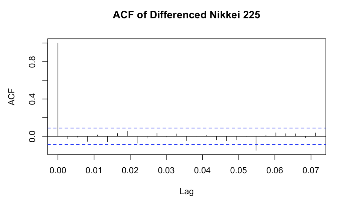
Figure 2: ACF of Differenced Nikkei 225(Picture Credit: Original)

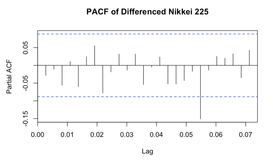
Figure 3: PACF of Differenced Nikkei 225(Picture Credit: Original)

3. Model Building

3.1. ARIMA Model

As Box and Jenkins said, the ARIMA model utilizes time series auto-correlation and trends to forecast stationary data in the short term [4]. We first used the ARIMA model to do the selection. Auto. Arima is employed to choose a better model that is considered by algorithms directly. In this process, the model chosen for the closing price of Nikkei225, respectively, is ARIMA (0,1,0). Analyzing the model's RMSE (root mean square error) is 455.7756, and the MAE (mean absolute error) is 296.4629, showing that the model's prediction error is notable and that it is limited in its capacity to capture short-term market movements. This could be due to significant market volatility and exogenous variables (such as international economic policy and geopolitical issues) that the model fails to account for. In conclusion, although the ARIMA(0,1,0) model might eliminate and smooth the trend in the data, the errors of the model indicate that it is of limited use for short-term forecasting.

3.2. Model Building

In this case, we first selected the ARIMA model again in order to improve the accuracy and robustness of the ARIMA model in financial market forecasting. Auto-regressive (AR) and moving average (MA) components are utilized to generate more complicated ARIMA models, such as ARIMA(1,1,1) or ARIMA(1,1,0). In addition, model selection and evaluation are performed by AIC and BIC. In comparison, the ARIMA(1,1,0) model performs better because its AIC value is 7424.93 and BIC value is 7433.327, both of which are lower than the numbers in the ARIMA(1,1,1) model, which have AIC = 7426.926 and BIC = 7439.522. In addition, I used check residuals to check whether ARIMA (1,1,0) was white noise and normal distribution in model diagnostician. The results are as follows:

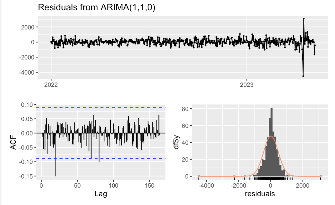
Figure 4: ACF and Histogram of residuals(Picture Credit: Original)

In Ljung-Box test, the p-value is 0.9931, higher than 0.05, and most of the lags are inside the range of critical values (two blue dashed lines) through ACF plot in Figure 4, so they are white noise. Furthermore, the histogram of residuals in Figure 4 shows that they are also normally distributed.

3.3. Model Forecasting

In this prediction of the Nikkei index based on the ARIMA (1,1,0) model, a comparison of the actual and predicted values shows that the model has a certain degree of accuracy in the short term. As shown in the figure, the red line represents the actual Nikkei index trend, the blue line is the forecast value, and the green dotted line indicates the 95% confidence interval. First of all, the root mean square error (RMSE) of the model is 455.61, indicating a relatively small error on the training set, which suggests that the model is a reasonable fit for the historical data. From the prediction results, the blue prediction line is basically stable in the next 30 days, indicating that the ARIMA model predicts little change in the index in the future, which is consistent with the short-term stabilization of the stock market. However, as the forecasting time increases, the confidence interval gradually widens which means the uncertainty increases. This reflects the limitations of the ARIMA model in long-term forecasting, especially in the face of market emergencies or major fluctuations, the model's prediction accuracy may be reduced (Figure 5).

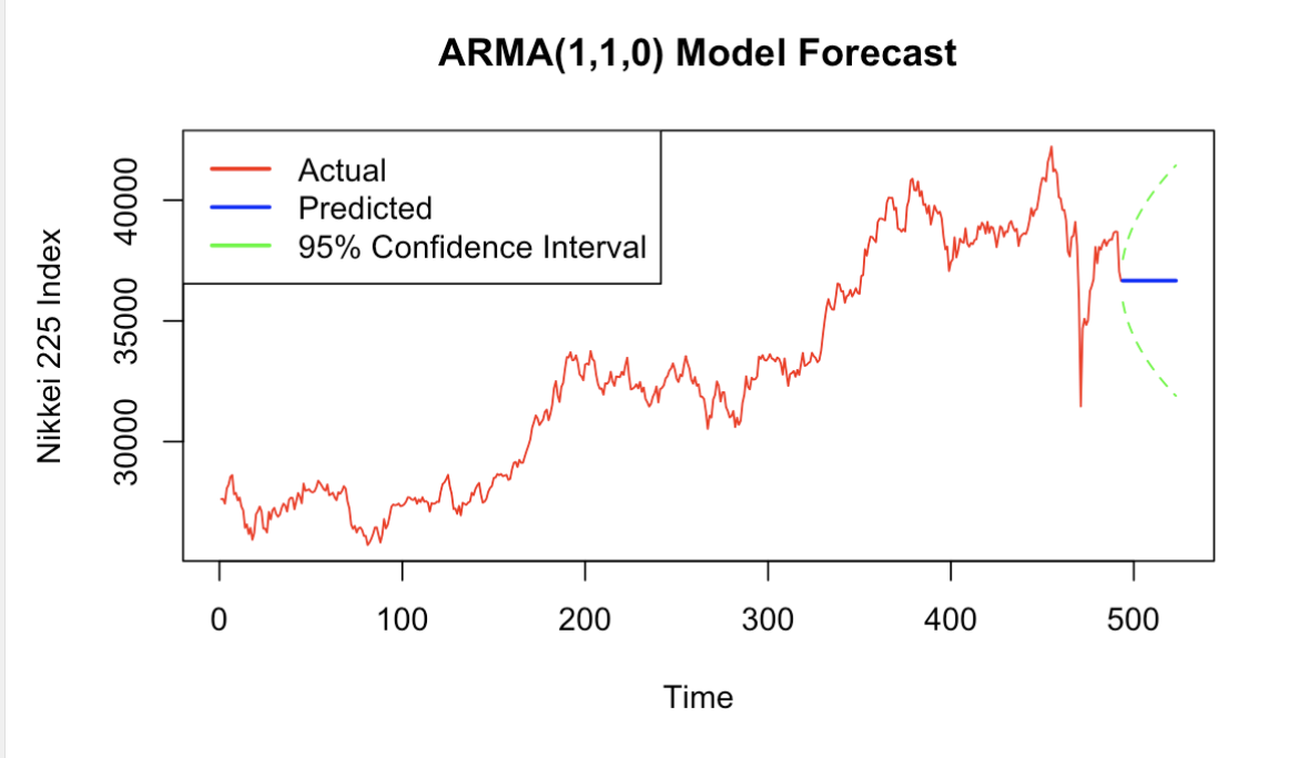
Figure 5: ARIMA(1,1,0) Model Forecast(Picture Credit: Original)

4. Result of the analysis

Overall, the ARIMA (1,1,0) model is able to capture the short-term trend of the Nikkei better, but its performance is more limited in more complex and volatile market environments like the sharp decline in the chart. The forecasting accuracy can be further improved in the future by introducing more external variables such as macroeconomic policies or using more complex models.

4.1. Suggestions

In his influential study on financial time series analysis, Tsay established that ARIMA models have found extensive use in short-term forecasting within financial markets, namely for unpredictable data like stock prices and interest rates. Nevertheless, Tsay also highlights that when dealing with complicated volatility in market data, such as the Nikkei index, it is often necessary to apply advanced models like GARCH (Generalized Auto-regressive Conditional Heterosexuality) or other diversity models, which are better equipped to manage volatility and offer more precise forecasts[5-7]. From my perspective, the findings of this study indicate that ARIMA models have demonstrated satisfactory accuracy in forecasting the short-term trends of the Nikkei index. However, the inherent volatility of the market implies that integrating more advanced models such as GARCH may provide even superior outcomes, particularly during times of significant market instability. To tell the truth, GARCH models have been particularly effective in predicting and modeling volatility clustering, which is known as a basic factor in financial time series data. There is research by Shamiri and Abu Hassan reveals that when it comes to predicting volatility in the stock market, GARCH models typically beat more conventional models such as ARIMA[7]. In addition, research has demonstrated that GARCH models are more effective at simulating conditional heteroskedasticity, as well as the time-varying volatility of financial returns, than ARIMA models are at capturing linear time series patterns[6][8]. Moreover, Miah and Rahman's research suggested that the ARIMA model has limitations when it comes to capturing the enduring volatility in financial markets[9]. Nevertheless, the GARCH model is a more dependable option for stock market forecasting since it is more adept at capturing both short- and long-term market volatility[10].

Additionally, Engle and Granger established the cointegration hypothesis, which states that when a long-term equilibrium relationship exists within a time series, integrating exogenous variables will significantly improve the accuracy of model prediction. Furthermore, this co-integration approach enables the modeling of long-term interactions between variables, which may be ignored by simpler models such as ARIMA model. In the context of this analysis, combining the ARIMA model with external macroeconomic indicators such as GDP growth and inflation rates could enhance the forecasting power of the Nikkei index for long-term trends [6]. As a result, while the ARIMA models provide a solid foundation for forecasting, future research may benefit from investigating these advanced models to capture the entire complexity of financial time series data.

5. Conclusion

In this study, the ARIMA (1,1,0) model was used for forecasting after ensuring the smoothness of the Nikkei 225 Index data by difference operation and ADF test. According to the model selection criteria of AIC and BIC, ARIMA (1, 1, 0) is considered the superior model. During the analysis of the diagram, the model shows some predictive ability in the short term, especially in predicting the trend in the next 30 days, which is more stable and consistent with the short-term stability of the stock market. However, the confidence intervals gradually widen over time, showing an increase in forecast uncertainty and limited model performance especially in the face of dramatic market volatility.

In conclusion, although the ARIMA model performs well in short-run financial market forecasting, the use of more advanced models such as GARCH may be more effective when dealing with complex volatile markets like the Nikkei. In addition, the inclusion of external macroeconomic variables such as the GDP growth rate and inflation rate can further enhance the model's long-run forecasting accuracy. Therefore, future research could dive into macroeconomic indicators' introduction or more sophisticated models' building in order to fulfill the grasp of long-term market trends.

References

[1]. Kutty, G. (2010). The relationship between exchange rates and stock prices: The case of Mexico. North American Journal of Finance and Banking Research, 4(4), 1-12.
[2]. Beltratti, A., & Morana, C. (2006). Breaks and persistency: Macroeconomic causes of stock market volatility. Journal of Econometrics, 131(1-2), 151-177.
[3]. BROCK, W., LAKONISHOK, J., & LeBARON, B. (1992). Simple Technical Trading Rules and the Stochastic Properties of Stock Returns. The Journal of Finance (New York), 47(5), 1731–1764. https://doi.org/10.1111/j.1540-6261.1992.tb04681.x
[4]. Box, G. E. P., & Jenkins, G. M. (1970). Time series analysis: Forecasting and control. Holden-Day.
[5]. Tsay, R. S. (2005). Analysis of Financial Time Series. In Analysis of Financial Time Series (Vol. 543). John Wiley & Sons, Incorporated.
[6]. Engle, R. F., & Granger, C. W. J. (1987). Co-Integration and Error Correction: Representation, Estimation, and Testing. Econometrica, 55(2), 251–276.
[7]. Shamiri, A., & Abu Hassan, S. (2007). Modeling and Forecasting Volatility of the Malaysian Stock Market. Journal of Applied Economic Sciences, 2(4), 123–128.
[8]. Bollerslev, T. (1986). Generalized Autoregressive Conditional Heteroskedasticity. Journal of Econometrics, 31(3), 307–327.
[9]. Miah, M., & Rahman, A. (2016). Modelling volatility of daily stock returns: Is GARCH(1,1) enough? American Academy of Science Research Journal of Engineering and Technology Science, 18(1), 29–39.
[10]. Nguyen Thi Hoang Anh, Tran Thi Thanh Huyen, Huynh Ngoc Kim Minh, & Nguyen Thi Ngoc Tran. (2018). Measuring volatility spillovers between developed and Southeast Asian emerging stock markets: a multivariate garch approach. Journal of International Economics and Management, 108, 65–88.
Cite this article
Gu,B. (2025). Forecasting the Index of Nikkei 225 Based on ARIMA Model. Advances in Economics, Management and Political Sciences,147,74-80.
Data availability
The datasets used and/or analyzed during the current study will be available from the authors upon reasonable request.
Disclaimer/Publisher's Note
The statements, opinions and data contained in all publications are solely those of the individual author(s) and contributor(s) and not of EWA Publishing and/or the editor(s). EWA Publishing and/or the editor(s) disclaim responsibility for any injury to people or property resulting from any ideas, methods, instructions or products referred to in the content.
About volume
Volume title: Proceedings of ICFTBA 2024 Workshop: Finance's Role in the Just Transition
© 2024 by the author(s). Licensee EWA Publishing, Oxford, UK. This article is an open access article distributed under the terms and
conditions of the Creative Commons Attribution (CC BY) license. Authors who
publish this series agree to the following terms:
1. Authors retain copyright and grant the series right of first publication with the work simultaneously licensed under a Creative Commons
Attribution License that allows others to share the work with an acknowledgment of the work's authorship and initial publication in this
series.
2. Authors are able to enter into separate, additional contractual arrangements for the non-exclusive distribution of the series's published
version of the work (e.g., post it to an institutional repository or publish it in a book), with an acknowledgment of its initial
publication in this series.
3. Authors are permitted and encouraged to post their work online (e.g., in institutional repositories or on their website) prior to and
during the submission process, as it can lead to productive exchanges, as well as earlier and greater citation of published work (See
Open access policy for details).