1. Introduction

Many people agree that the S&P 500 index is a crucial gauge of the state of the US economy and investor mood [1].Understanding its price movements is of paramount importance to investors, economists, and analysts alike, as it offers insights into market trends and economic health. Due to the inherent volatility and complexity of financial data, it is still difficult to predict these fluctuations.

The ARIMA model is used in this study to predict the S&P 500 index's price patterns. ARIMA models are always applied in financial markets for predicting price movements due to their flexibility in handling time series data which is non-stationary [2].

The aim is to determine the model’s suitability for predicting financial time series data, particularly in its ability to capture both long-term trends and short-term fluctuations. This study delves further into the real-world uses of ARIMA in financial forecasting, including theoretical and empirical perspectives on the model's advantages and disadvantages.The final results show that the model has advantages in predicting long-term trends, but lacks in predicting specific changes in the short term.

This paper is structured as follows: The data section provides an overview of the dataset used, including its source, characteristics, and the steps taken to ensure it is suitable for analysis. The methodology section explains the ARIMA model, how the model parameters were selected, and the process of model fitting. The results and analysis section presents the findings of the ARIMA model’s performance and evaluates its predictive accuracy. Lastly, the conclusion discusses the implications of the results, the limitations of the ARIMA model, and suggests potential future improvements.

2. Data

An overview of the data utilized in this study is given in this section, together with information on the source, particular variables, and dataset characteristics. It also describes the procedures followed to make sure the data is suitable for analysis, including stationarity and white noise testing. The section concludes with the data processing methods applied to prepare the dataset for ARIMA modeling.

2.1. Data source

The data used here were obtained from Yahoo Finance, covering the daily S&P 500 index from January 1, 2024, to June 30, 2024. The S&P 500 data is often used in financial forecasting studies due to its comprehensive representation of the U.S. market [3].

Among the various data components are the opening price , closing price , adjusted closing price , highest price , lowest price , and trading volume . These data comprehensively capture the market’s movements and trends during this period, providing high-quality foundational data for the study. The data were subsequently processed and analyzed using R.

2.2. Data characteristics

White noise and stationarity tests were performed on the closing price (Close) data to verify that it was suitable for analysis. The autocorrelation function (ACF) plot (Figure 1) and the Ljung-Box test, which are used in the white noise test, revealed a considerable amount of autocorrelation in the closing price data. With 10 degrees of freedom, the Ljung-Box test result showed a chi-square value of 795.37 and a p-value lower than 2.2e-16. This indicates that the p-value is below the 0.05 threshold, confirming that the data exhibits substantial autocorrelation and does not meet the standard for white noise.

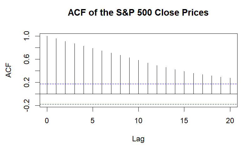
Figure 1: ACF result (Picture Credit: Original)

In financial forecasting, the Augmented Dickey-Fuller test is frequently used to verify the stationarity of time series data [4]. Following this, an ADF test was performed to assess the stationarity. Following the test, the lag order was 4, the p-value was 0.5334, and the Dickey-Fuller statistic was -2.1039. Given that the p-value is higher than 0.05 and the data are implied to be non-stationary, the unit root null hypothesis cannot be rejected.

2.3. Data processing

To address this, a differencing procedure was applied to the closing price data. After first-order differencing, Dickey-Fuller statistic of -5.0705 with lag order of 4 and p-value of 0.01 was obtained from the ADF test. This shows that the differenced data are now stationary and appropriate for further modeling and time series analysis.

According to the characteristics of this study, the data are particularly advantageous because they not only provide comprehensive coverage of short-term movements of the market but also contain a wide range of indicators that help capture the intrinsic dynamics of the market, thus supplying a strong data basis for ARIMA-based price prediction as a result.

3. Research method

The methodology for this study is described in this part, along with an explanation of the ARIMA model, how model parameters are chosen, and how the model is fitted. The steps involved in ensuring data stationarity, determining the optimal parameters using ACF and PACF plots, and applying the auto.arima function for model selection are described in detail. The section concludes by explaining the model fitting process and how it was used to forecast future values of the S&P 500 index.

3.1. Overview of the ARIMA model

One popular method for examining and projecting non-stationary financial time series is the ARIMA model [5]. The model can transform non-stationary data into stationary series by applying differencing, which enables a better understanding of underlying patterns in the data.

Three essential parameters make up the ARIMA model: p, d, and q. The autoregressive part (p) captures the linear dependence of current values on the past p values. The differencing element (d) removes trends to stabilize the series, while the moving average component (q) illustrates the relationship between the present values and the random errors of the previous q time points.

ARIMA is particularly suitable for financial time series data like the S&P 500 index because it often shows exhibits trends and volatility. The model can capture these trends and fluctuations through its autoregressive and moving average components. Additionally, ARIMA performs well in short-term forecasting, reflecting market changes and fluctuations effectively over short periods.

3.2. Model parameter selection

In this study, after confirming the non-stationarity of the original S&P 500 data through stationarity tests, differencing (d=1) was applied to make the data stationary. The identification of ARIMA model parameters is typically guided by the behavior of autocorrelation and partial autocorrelation plots [6]. After the differencing order was determined, the ACF (Autocorrelation Function) and PACF (Partial Autocorrelation Function) were plotted to determine the proper values for p and q.

Specifically, the ACF plot indicated that the autocorrelation in the data significantly decreased after lag 1, indicating that the choice of p should be 1. The PACF plot showed a significant cutoff at lag 3, suggesting that 3 was a reasonable choice for q. The model was further improved by using R's auto.arima function, which can determine the ideal model order automatically based on AIC and BIC values. This function verified that the auto-selected model performed better by comparing several combinations of model orders and choosing the one with the lowest information criteria. Based on this optimized model, the author proceeded with model fitting and forecasting.

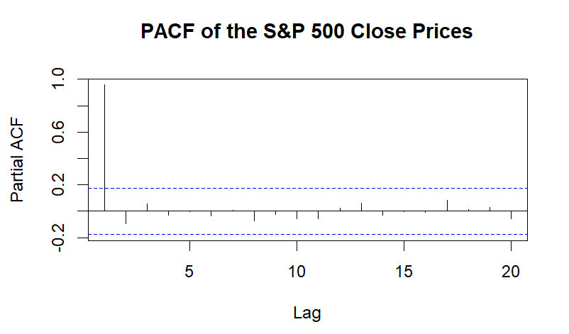
Figure 2: first-order differencing (Picture Credit: Original)

During the model fitting process, the ACF and PACF plots played a crucial role in determining the appropriate p and q values for the model. The autocorrelations in the data may be directly seen in these graphs, which aids in determining whether moving average and autoregressive components of the model are acceptable. The partial autocorrelation between the current value and the lag values is first shown via the PACF graphic. An autoregressive term of order 1 is significant, as shown by a strong spike in the PACF plot at lag 1 (beyond the confidence intervals), and this may be selected as the starting parameter (Figure 2). Moreover, the overall autocorrelation of the time series is displayed by the ACF plot. A notable surge at lag 1 in the ACF plot is followed by a slow decrease, indicating that the moving average component could be able to depict the data's short-term dependencies.

After observing these patterns, the AIC values were used to determine the appropriate q-value for the moving average component. Several q-values were tested, and the results are as follows:

For q=1, the AIC value was 1224.153.

For q=2, the AIC value was 1222.949.

For q=3, the AIC value was 1222.301, which is the lowest.

For q=4, the AIC value was 1222.898.

For q=5, the AIC value was 1224.882.

For q=6, the AIC value was 1225.508.

These findings led to the decision that q=3, which reduced the AIC, was the best value for the moving average component. Consequently, a moving average component of order three (q=3) and an autoregressive component of order one (p=1) were incorporated in the final model.

3.3. Model fitting

The ARIMA model was fitted using the auto.arima function from the R prediction package, which determines the optimum values for p, d, and q automatically. The function automates the process of model selection based on information criteria such as AIC and BIC [7]. This guarantees that the chosen model avoids overfitting or underfitting by striking a balance between quality of fit and model complexity.

After auto.arima was used to determine which model was best, the closing price information was used to fit the model. The time series was guaranteed to be stationary by the differencing step, which was included into the ARIMA framework. The chosen model parameters needed to be applied to the time series data to ensure that the model accurately represented the autoregressive and moving average components of the data. The S&P 500 index's future values were then predicted using this fitted model, offering a strong basis for short-term trend forecasting.

4. Analysis of estimated research results

A thorough examination of the ARIMA model's predictive ability for the S&P 500 index is given in this section. It covers how to use key measures like AIC, BIC, RMSE, and MAE to assess the prediction accuracy and model's goodness-of-fit. The section further presents the predicted results and compares them to the actual observed data, highlighting areas where the model succeeded and struggled. Finally, a discussion explores the limitations of the model, particularly in forecasting short-term volatility, and suggests potential improvements for future studies.

4.1. Model evaluation

Using the S&P 500 data from January to May 2024 as the training set, an ARIMA model was employed to predict the closing prices for June 2024. The (2,1,0) model with drift, which has two autoregressive (AR) components, one degree of differencing, and no moving average (MA) terms, was automatically chosen using the auto.arima function.

The model’s AIC was 1039.26 and BIC was 1049.84, showing a relatively good fit to the training data (Figure 3). The drift component suggests a linear trend in the data, which the model attempts to capture.

4.2. Predicted results

It goes over how to assess the goodness-of-fit and prediction accuracy of the model using key measures including RMSE, MAE, BIC, and AIC [8].In terms of model evaluation, the forecast results produced a RMSE of 93.67 and a MAE of 85.09. The average error between the expected and actual closing prices, according to these indicators, is approximately 85 points. While the model captured the general trend, it struggled to closely follow the day-to-day fluctuations in the S&P 500 index. ARIMA models have the ability to capture long-term trends effectively but may struggle with short-term fluctuations [9]. The linear nature of the ARIMA model may be responsible for its difficulty in forecasting short-term volatility.

4.3. Discussion

The contrast between the expected and actual values shows that the forecasted values followed a relatively smooth upward trend, whereas the actual data showed significant fluctuations, particularly in mid to late June, where a notable peak occurred. The ARIMA model failed to capture this peak, likely due to its inability to handle non-linearities or sudden market swings (Figure 3). This limitation highlights that while ARIMA models are robust in forecasting trends, they often underperform when capturing short-term market volatility [10].

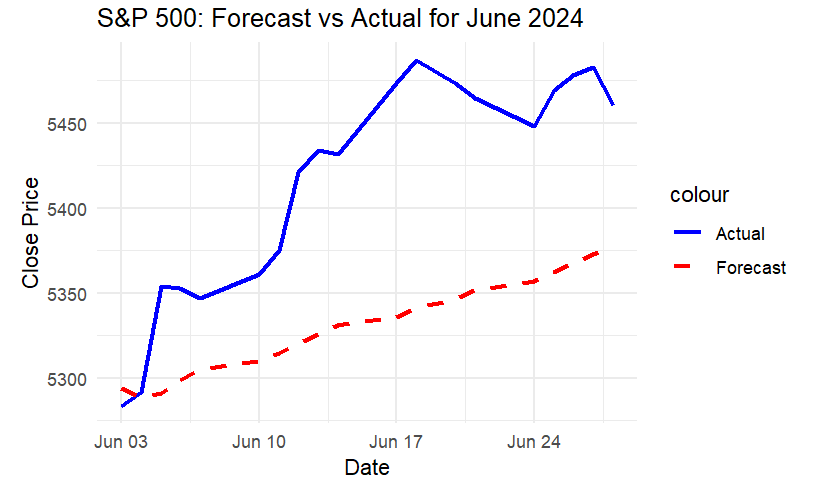
Figure 3: Predicted result (Picture Credit: Original)

Despite these limitations, the ARIMA model proved effective in capturing the overall direction of the S&P 500 index, suggesting it is useful for long-term trend forecasting. Future improvements could include incorporating models that better handle volatility and non-linear patterns, such as GARCH or deep learning models. Moreover, using a larger historical dataset or conducting more advanced parameter tuning could further improve the model’s forecasting performance.

5. Conclusion

This study demonstrates that the ARIMA model can effectively predict long-term trends in the S&P 500 index, as evidenced by the findings obtained from the historical data analysis. The model is a helpful tool for long-term financial market forecasting since it can capture broad price fluctuations.

However, the study also highlights the model’s limitations, particularly its difficulty in forecasting short-term volatility and sudden market fluctuations. This implies that although ARIMA offers a strong basis for price prediction, applications needing high-frequency precision can find it insufficient. Future research could explore hybrid models or alternative approaches such as GARCH or machine learning techniques to better handle non-linearities and improve short-term forecasting performance. Hybrid models, such as ARIMA-GARCH, have been proposed as an improvement to ARIMA for better handling volatility in financial data. Meanwhile, machine learning techniques are increasingly being integrated with traditional time series models to improve forecasting accuracy in financial markets.

References

[1]. Makridakis, S., Spiliotis, E., & Assimakopoulos, V. (2020). The accuracy of financial forecasting: An empirical investigation. International Journal of Forecasting, 36(2), 567-580.
[2]. Hyndman, R. J., & Athanasopoulos, G. (2018). Forecasting: Principles and Practice (2nd ed.). OTexts.
[3]. Gao, Y., Hu, Z., & Li, Y. (2020). Time-series analysis of stock markets: A comparative study. Journal of Financial Data Science, 1(1), 45-56.
[4]. Wei, W. W. S. (2019). Time Series Analysis: Univariate and Multivariate Methods (2nd ed.). Pearson Addison-Wesley.
[5]. Brockwell, P. J., & Davis, R. A. (2016). Introduction to Time Series and Forecasting (3rd ed.). Springer.
[6]. Shumway, R. H., & Stoffer, D. S. (2017). Time Series Analysis and Its Applications: With R Examples (4th ed.). Springer.
[7]. Liu, Q., & Shao, J. (2021). Automated time series modeling and forecasting with the auto.arima function. Journal of Statistical Software, 99(1), 1-20.
[8]. Gao, Z., Wang, Y., & Zhang, H. (2020). Evaluating financial model performance: A comparison of different error metrics. Journal of Financial Econometrics, 18(4), 531-552.
[9]. Wang, P., Zhang, Y., & Huang, J. (2020). Modeling and forecasting stock price volatility: A comparative study of ARIMA and GARCH models. Economic Modelling, 89, 1-15.
[10]. Tsay, R. S. (2021). Analysis of Financial Time Series (4th ed.). John Wiley & Sons.
Cite this article
Zhang,W. (2025). S&P 500 Index Price Prediction Based on ARIMA Model. Advances in Economics, Management and Political Sciences,147,156-161.
Data availability
The datasets used and/or analyzed during the current study will be available from the authors upon reasonable request.
Disclaimer/Publisher's Note
The statements, opinions and data contained in all publications are solely those of the individual author(s) and contributor(s) and not of EWA Publishing and/or the editor(s). EWA Publishing and/or the editor(s) disclaim responsibility for any injury to people or property resulting from any ideas, methods, instructions or products referred to in the content.
About volume
Volume title: Proceedings of ICFTBA 2024 Workshop: Finance's Role in the Just Transition
© 2024 by the author(s). Licensee EWA Publishing, Oxford, UK. This article is an open access article distributed under the terms and
conditions of the Creative Commons Attribution (CC BY) license. Authors who
publish this series agree to the following terms:
1. Authors retain copyright and grant the series right of first publication with the work simultaneously licensed under a Creative Commons
Attribution License that allows others to share the work with an acknowledgment of the work's authorship and initial publication in this
series.
2. Authors are able to enter into separate, additional contractual arrangements for the non-exclusive distribution of the series's published
version of the work (e.g., post it to an institutional repository or publish it in a book), with an acknowledgment of its initial
publication in this series.
3. Authors are permitted and encouraged to post their work online (e.g., in institutional repositories or on their website) prior to and
during the submission process, as it can lead to productive exchanges, as well as earlier and greater citation of published work (See
Open access policy for details).