1. Introduction

The stock market plays an indispensable role in the global economy as it allows money to flow through the market and creates liquidity for businesses and companies. It facilitates the capital raising of companies and simultaneously provides the investors with opportunities to earn profits through dividends and selling their stocks. However, there is also a risk that the investors will incur losses if the stock price declines. A part of this risk, on the other hand, can be diminished through diversification, a risk management strategy that involves allocating capital to a variety of assets. As such, an investment portfolio that combines diverse financial assets, including stocks and bonds, is created to guarantee that the assets are preserved. Therefore, the topic of finding optimized investment portfolios under different circumstances has been in the limelight for an extended period.

First proposed by Harry Markowitz in 1952, the Markowitz Model successfully addressed the puzzle of portfolio optimization by maximizing the return at a given range of risks [1]. However, the calculation process introduced in the model is rather complicated as it involves a significant number of estimates. Therefore, people tried to improve the model on its original basis. In 1963, William Sharpe proposed the Single Index Model, a model that largely simplified the Markowitz Model [2].

Some scholars have already utilized both the Markowitz Model and the Index Model to analyze the investment portfolios formed by different stocks. In 2020, Putra et al. presented a study of the different performances of the optimal portfolios yielded from the Markowitz Model and the Index Model. They found that while the portfolio optimized by the Index Model performs better than that of the Markowitz Model, there is no statistically significant difference between the average returns yielded from the two models [3]. In a similar study, Cao established that the Index Model can be considered a feasible approximation of the Markowitz Model in practical applications when the number of risky assets increases in a portfolio [4]. In a 2022 investigation, by comparing the results of applying both models to the selected portfolio, Ni also mentioned the marginal improvements in the performance of the Index Model and advised the investors targeting the Hong Kong stock market to opt for the Index Model over the Markowitz Model when optimizing their portfolios [5]. In the same year, Qin conducted research to compare the impact of the two models on the portfolio formed by stocks specifically from the Chinese stock market. The research set up an additional optimization constraint to ensure that the weight of each risky asset is non-negative, simulating the relevant policy that the Chinese stock market does not allow short selling. Similar to the conclusion drawn by Putra et al., Qin also concluded that under such optimization constraint, while both the Markowitz Model and the Index Model can effectively diversify the specific risk, the Index Model performed better than the Markowitz Model when comparing the Capital Allocation Line (CAL), Minimum-Variance Portfolio, etc. [6]. On the other hand, Zhang chose to analyze the American stock market using the same models but introduced more constraints to simulate different real-life situations in the optimization process. Eventually, he concluded that both the portfolios optimized by the Markowitz Model and the Index Model possess similar Sharpe ratios despite the asset allocation in the two portfolios being very different. Just like Cao, they also pointed out that the reduced complexity of the Index Model makes it preferable when the number of assets increases in a portfolio [7]. Furthermore, Qu et al. also analyzed the performances of the two models under these additional optimization constraints. They arrived at the conclusion that under the first three conditions, the portfolio optimized by the Markowitz Model consistently outperformed in predicting the Minimum Variance Portfolio, whereas the portfolio optimized by the Index Model overtook in predicting the Maximum Sharpe Ratio Portfolio. Yet they found that this discrepancy vanished under other optimization constraints, where the Index Model generally demonstrated superior performance [8]. This paper will also use their studies as a reference and conduct similar research based on the same five optimization conditions.

This paper aims to analyze the difference between the Markowitz Model and the Index Model by finding and comparing the optimal investment portfolio formed by a riskless asset – the 1-month Fed Funds Rate – and eleven risky assets, including ten stocks and one equity index, the S&P 500 index using these two models. This paper first obtains the historical data of the securities from the past 20 years and aggregates the daily data to monthly returns to avoid the non-Gaussian effect in the calculation. Then, the correlation matrix that displays a cross Pearson correlation coefficient between each pair of securities will be generated. Finally, utilizing Python, the weight of each security in the optimized portfolio according to the Markowitz Model and the Index Model under the five scenarios can be derived. This paper analyzes the strengths and weaknesses of each model under different schemes by comparing the total returns, risks (standard deviations), and reward-to-volatility rate (Sharpe Ratio) of each portfolio.

2. Data and Methodology

2.1. The Markowitz Model

The Markowitz Model is a prevalent portfolio optimization model first proposed by Henry Markowitz in 1952. It is the foundation of the Modern Portfolio Theory as it analyzes different potential combinations of a given set of securities and determines the optimal portfolios by maximizing the returns for a given risk. The portfolio selection approach, according to the Markowitz Model, includes three steps as follows.

Firstly, Determine the risk-return opportunities available for investors. With the expected returns on the Y-axis and standard deviations (risk) on the X-axis, all the combinations can be represented in the plot. Determine the Minimum-Variance Frontier, the graph of the lowest possible variance (risk) that can be attained from a given portfolio return. All individual assets, or portfolios composed of a single asset, lie to the right of the Minimum-Variance Frontier and are considered sub-efficient. The part of the Minimum-Variance Frontier that is above the Global Minimum Variance portfolio is known as the Efficient Frontier of risky assets, which provides the best risk-return combinations.

Secondly, identify the Capital Allocation Line (CAL) with the highest Reward-to-Volatility ratio (Sharpe ratio) and establish the optimal risky portfolio. The Capital Allocation Line is the graph that displays the possible returns investors may receive by taking on certain levels of risk. The Capital Allocation Line can be expressed as

\( CAL: E({R_{C}})={R_{f}}+{S_{P}}\cdot {σ_{C}} \) (1)

where \( f \) denotes the riskless portfolio, \( P \) denotes the risky portfolio, and C denotes the complete portfolio, i.e., the combination of the risky and riskless portfolios. The vertical intercept \( {R_{f}} \) , therefore, represents the risk-free rate, i.e., the expected rate of return from the riskless assets; \( {σ_{C}} \) denotes the standard deviation or the risk of the complete portfolio; and its slope, \( {S_{P}} \) , is the Sharpe ratio. To be more specific, the Sharpe ratio can be expressed as

\( {S_{P}}=\frac{E({R_{P}})-{R_{f}}}{{σ_{P}}} \) (2)

which indicates the excess return the investors receive for each additional unit of risk. As a result, seek the CAL with a larger Sharpe Ratio as it signifies higher returns relative to the same amount of risk. Plotting both the CAL and the Efficient Frontier on the same graph, the optimal risky portfolio P corresponds to the point where the CAL is tangent to the Efficient Frontier. P corresponds to the point where the CAL is tangent to the Efficient Frontier.

Selecting the appropriate combination with the riskless portfolio. After constructing the optimal risky portfolio, the complete portfolio can be calculated, taking into consideration the investor’s degree of risk aversion. The risk aversion coefficient, A, is introduced to quantify the risk aversion degrees of different investors. \( A \gt 0 \) for risk-averse investors who loathe taking any risks; \( A=0 \) for risk-neutral investors whose Utility ( \( U \) ) won’t be affected by the changes in risk; and A\ <\ 0 for risk-seeking investors who are more willing to take risks. The proportion of the complete portfolio to be invested in the risky portfolio, \( y \) , can be expressed as

\( y=\frac{E({R_{P}})-{R_{f}}}{A\cdot σ_{P}^{2}} \) (3)

leaving \( (1-y) \) to be invested in the riskless portfolio.

Let \( \vec{μ}={\lbrace μ_{1}},…,{{μ_{n}}\rbrace ^{T}} \) denote the set of average returns of the instruments; \( \vec{w}=\lbrace {w_{1}},…,{w_{n}}{\rbrace ^{T}} \) represent the set of weights of the instruments; \( \vec{σ}=\lbrace {σ_{1}},…,{σ_{n}}{\rbrace ^{T}} \) denote the set of standard deviations of the instruments; \( \vec{v}=\lbrace {w_{1}}{σ_{1}},…,{w_{n}}{σ_{n}}{\rbrace ^{T}} \) be an auxiliary vector; and finally let

\( P = (\begin{matrix}{ρ_{11}} & ⋯ & {ρ_{1n}} \\ ⋮ & ⋱ & ⋮ \\ {ρ_{n1}} & ⋯ & {ρ_{nn}} \\ \end{matrix}) \) (4)

Be the correlation matrix that displays the cross-correlation coefficient between instruments. The return of the risky portfolio based on the Markowitz Model can be expressed as \( {R_{P}}=\vec{w}\cdot \vec{μ}=\vec{w}{\vec{μ}^{T}}, \)

whereas the portfolio risk is \( {σ_{P}}=\sqrt[]{\vec{v}P{\vec{v}^{T}}}. \)

2.2. The Index Model

Despite the Markowitz Model being a prominent model in portfolio optimization, it requires an enormous amount of estimates of expected returns, variances, and covariances. Suppose a security analyst is to analyze n stocks in a portfolio, then he needs to produce n estimates of expected returns, n estimates of variances, and \( ({n^{2}}-n)/2 \) estimates of covariances. Therefore, a total of \( ({n^{2}}+3n)/2 \) estimates are required for calculation. Yet, no specific approach has been demonstrated by the Markowitz Model to produce these estimates. The only speculation one can make is to use historical data although sometimes past returns may be unreliable. As a result, the Index Model, first introduced by William Sharpe in 1963, which also optimizes investment portfolios by balancing risks and returns, has, to a large extent, simplified the Markowitz Model as it only requires \( 3n + 2 \) predictions to be made.

In the Index Model, a market index, such as the S&P 500, has been used as a proxy for the macroeconomic factor that accounts for the systematic risk that cannot be diversified. Then, the excess return of a security, \( {R_{i}}={r_{i}}-{r_{f}} \) , has been regressed on the excess return of the market index, \( {R_{M}}={r_{m}}-{r_{f}} \) . The historical data \( {R_{i}}(t) \) and \( {R_{M}}(t) \) are collected where t denotes the date of each paired observation. The regression equation can be expressed as

\( {R_{i}}(t)={α_{i}}+{β_{i}}\cdot {R_{M}}(t)+{e_{i}}(t) \) (5)

The intercept of this equation, \( {α_{i}} \) is the expected excess return of the security when the market excess return is 0. The slope, \( {β_{i}}, \) demonstrates the sensitivity of the security to the index: it is the change in security return for every \( 1\% \) float in the return of the index. \( {e_{i}} \) is the residual of the security return due to firm-specific surprise where \( {e_{i}}∼N(0,{σ^{2}}) \) . As a result, by taking the expectation on both sides of the equation, then obtain \( E({R_{i}})={α_{i}}+{β_{i}}\cdot E({R_{M}}), \) which demonstrates the relationship between the expected return of a security and the market risk premium.

Similarly, the risk of a security can be divided into two parts – the firm-specific risk, \( {σ^{2}}({e_{i}}) \) , and the market risk that can be diversified, \( β_{i}^{2}σ_{M}^{2} \) . Therefore, the variance of a security is \( σ_{i}^{2}=β_{i}^{2}σ_{M}^{2}+{σ^{2}}({e_{i}}). \)

Likewise, the returns and risks can be expressed in the vector form by letting \( \vec{β}=\lbrace {β_{1}},…,{β_{n}}{\rbrace ^{T}}. \) Similar to the equations mentioned above for the Markowitz Model, the return of the risky portfolio calculated by the Index Model can be expressed by \( {R_{P}}=\vec{w}\cdot \vec{μ}=\vec{w}{\vec{μ}^{T}}. \) In contrast, the risk can be expressed as \( {σ_{P}}=\sqrt[]{{({σ_{M}}{β_{P}})^{2}}+\sum _{1}^{n}w_{i}^{2}{σ^{2}}({ϵ_{i}})}, \) where \( {β_{P}}=\vec{w}{\vec{β}^{T}} \) denotes the portfolio beta. Furthermore, since correlation is an important aspect of diversification, and \( {r_{xy}}=\frac{Cov({r_{i}},{r_{j}})}{{σ_{x}}\cdot {σ_{y}}}, \) The covariance can be determined by the beta coefficients, where \( Cov({r_{i}},{r_{j}})={β_{i}}{β_{j}}σ_{m}^{2}. \)

2.3. Stock Selection

This paper chooses the investment portfolio formed by a proxy for the risk-free rate (1-month Fed Funds Rate) and a total of eleven risky assets, including one equity index (S&P 500) and ten stocks that belong in groups to four different sectors according to Yahoo Finance. The stocks selected are listed as follows:

• Technology

• Apple Inc. (AAPL): a technology company headquartered in Cupertino in Silicon Valley that manufactures and sells electronics, software, and services.

• NVIDIA Corp. (NVDA): an American multinational technology company that mainly specializes in Graphics Processing Units (GPU).

• Microsoft Corp. (MSFT): a technology corporation headquartered in the United States that’s best known for its software and related products.

• Financial Services

• Bank of America Corp. (BAC): an investment bank and financial services firm in the US. It’s the second-largest banking institution globally in terms of market capitalization.

The Goldman Sachs Group, Inc. (GS), an investment bank and financial services company founded in 1869, and is the world's second-largest investment bank by revenue.

• JPMorgan Chase & Co. (JPM): a multinational finance company founded in New York City, as well as the world’s largest bank measured by market capitalization.

• Industrial

• Boeing Co. (BA): one of the largest aircraft manufacturers in the world that designs, develops, manufactures, and supports jetliners, military aircraft, satellites, defense, etc.

• FedEx Corp. (FDX): an American conglomerate holding company that mainly provides transportation and delivery services around the globe.

• Healthcare

• Johnson & Johnson (JNJ): an innovative pharmaceutical, biotechnology, and medical technologies corporation headquartered in New Jersey.

• Merck & Co. (MRK): a multinational advanced pharmaceutical company that was first founded in Germany and is now headquartered in the United States.

2.4. Optimization Constraints

The companies listed in the above section are some of the leading corporations in their fields. As they belong to different industries, the unsystematic risk should theoretically be reduced to a certain extent. This paper will utilize both the Markowitz Model and the Index Model to find the optimized investment portfolio under five different cases of constraints that simulate various real-life scenarios. The five cases are listed as follows:

• Without any additional optimization constraints.

• \( Σ_{i=1}^{11}|{W_{i}}|≤2 \) : This extra optimization constraint is set up to simulate the Regulation T, established by the Financial Industry Regulatory Authority (FINRA). It specifies that an investor can borrow up to 50% of the purchase price from the broker-dealers.

• \( |{W_{i}}|≤1,∀i∈[1,11] \) : This additional optimization constraint is designed to simulate some random arbitrary box constraints on weights.

• \( |{W_{i}}|≥0,∀i∈[1,11] \) : This additional optimization constraint is intended to mimic the typical limitations in the United States mutual fund industry since the open-ended mutual funds in the U.S. are not allowed to have any short positions.

• \( {W_{1}}=0 \) : This additional optimization constraint is for us to test whether the inclusion of the broad index into investment portfolio has any impact.

2.5. Data Processing

Obtain the recent 20 years of historic daily total return data of the ten stocks, the S&P 500 index, and the 1-month Fed Funds from September 17, 2024, to September 20, 2024. However, it can be easily noticed that the observations of each stock vary due to different trading days and public holidays. Furthermore, an underlying assumption for all classical finance problems states that the log returns of the stocks should be independent and normally distributed.

Regardless, as shown in Figure 1, the log returns of all the securities do not follow a Gaussian distribution as the plot displays extremely fatter tails on both sides or in other words, demonstrates significant kurtosis. The conclusion is similar in table 1.

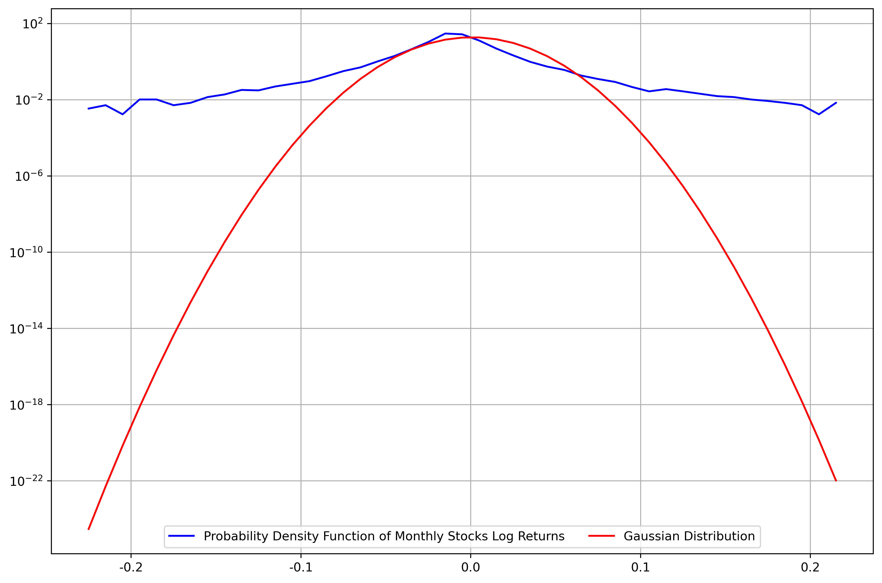
Figure 1: Probability distribution of daily log returns of securities versus Gaussian distribution.

Table 1: Test statistics of daily returns.

As a result, it is necessary to aggregate the data before proceeding to calculate the optimized portfolio under each constraint to minimize the non-Gaussian effect. According to multiple trials, the paper finds that aggregating the daily data into both monthly data and yearly data are feasible option. Nonetheless, the latter approach would significantly reduce the number of observations available since the interval is excessively large; this paper chooses to aggregate the data into monthly observations.

Table 2: Test statistics of monthly returns.

As can be seen from Table 2, the kurtosis of each security has reduced substantially compared to those of the daily returns. The statistical calculation can also be confirmed visually by plotting the probability distribution of the monthly log returns of the indices and stocks and comparing it with the Gaussian distribution – as shown in Figure 2, both tails are contained within an acceptable range from the real Gaussian distribution, and the log returns roughly follow a Normal distribution.

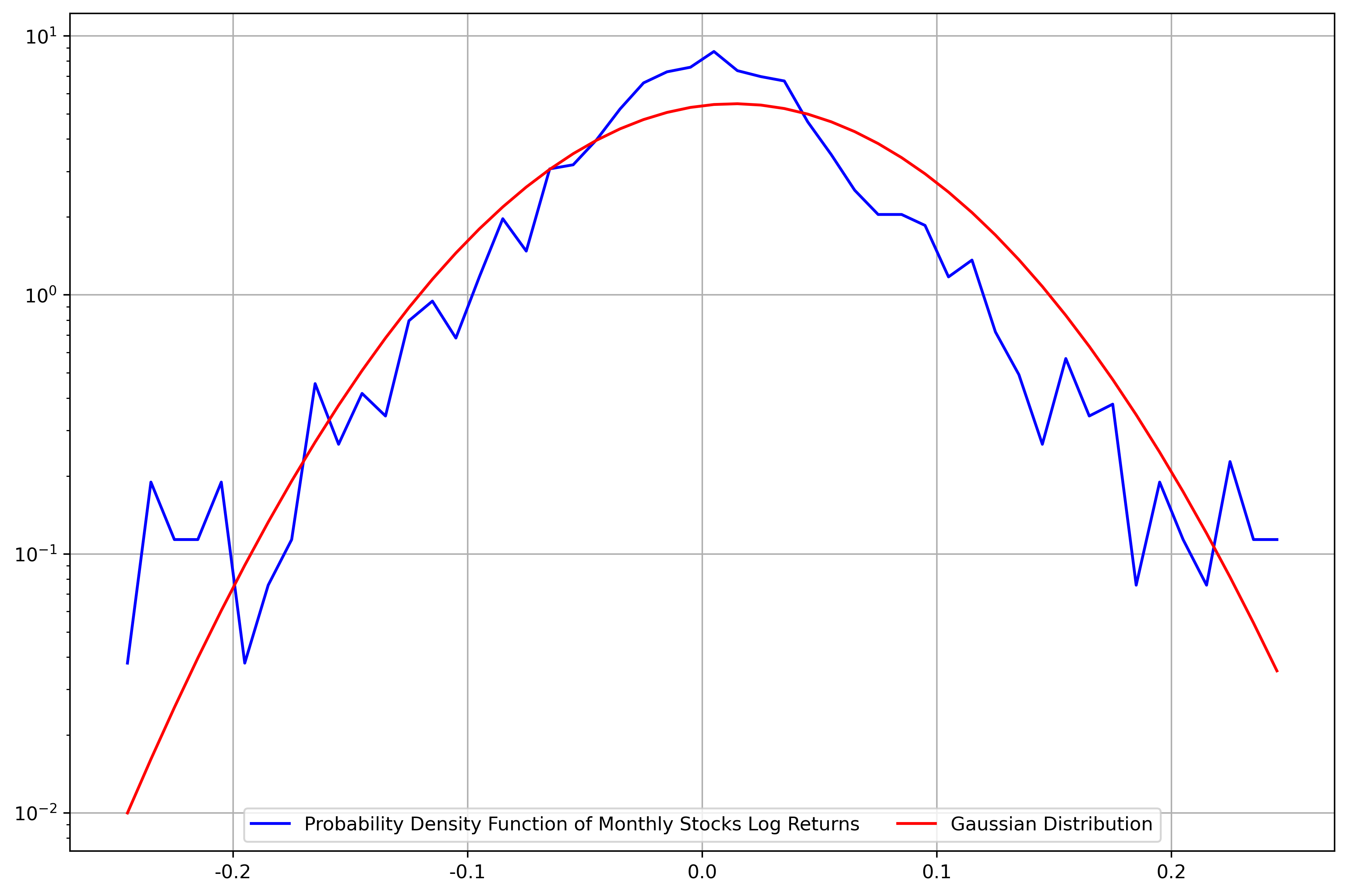
Figure 2: Probability distribution of monthly log returns of securities versus Gaussian distribution.

2.6. Correlation Analysis Between Securities

As introduced in both the Markowitz Model and the Index Model earlier, the cross-correlation coefficient between each pair of securities is rather vital as it plays an intensive role in portfolio diversification. According to the Modern Portfolio Theory (MPT), portfolios formed by securities with negative correlations are always preferred because the total risk is reduced as the positive and negative returns cancel out. The Pearson correlation between each pair of securities is generated as figure 3.

Figure 3: Correlation Matrix of Securities.

3. Results and Analysis

3.1. Optimized Portfolios Without Constraints

As mentioned above, the first scenario this paper discusses is a “free” problem where no specific constraints are applied, and thus, the area of permissible portfolios in general can be illustrated. The results also impart a basic understanding of the distinction between the portfolios produced by the Markowitz Model and the Index Model.

Table 3: Optimized risky portfolio without constraints using the Markowitz Model.

Table 4: Optimized risky portfolio without constraints using the Index Model.

Table 3 and Table 4 show the results of 2 optimized investment portfolios, the Minimum Variance Portfolio and the Maximum Sharpe Ratio Portfolio, obtained using the Markowitz Model and the Index Model, respectively. For the Minimum Variance Portfolio, the Index Model seems to have produced a portfolio with a relatively smaller risk yet with a lower Sharpe ratio. On the other hand, both models provided similar results in optimizing the Maximum Sharpe Ratio portfolio. The Index Model produced a portfolio with a Sharpe ratio of 1.61, whereas the Markowitz Model produced a portfolio with a slightly higher Sharpe ratio of 1.66. As a result, under the scenario of no additional constraint, both the Markowitz Model and the Index Model performed well, with the Markowitz Model performing slightly better due to the higher Sharpe ratio. It becomes more intuitive when both portfolio frontiers are plotted and superimposed as shown in Figure 4. The frontiers of the Markowitz Model are higher yet to the left in the graph compared to those of the Index Model; the Capital Allocation Line (CAL) of the Markowitz Model also has a steeper slope, which signifies a larger Sharpe Ratio.

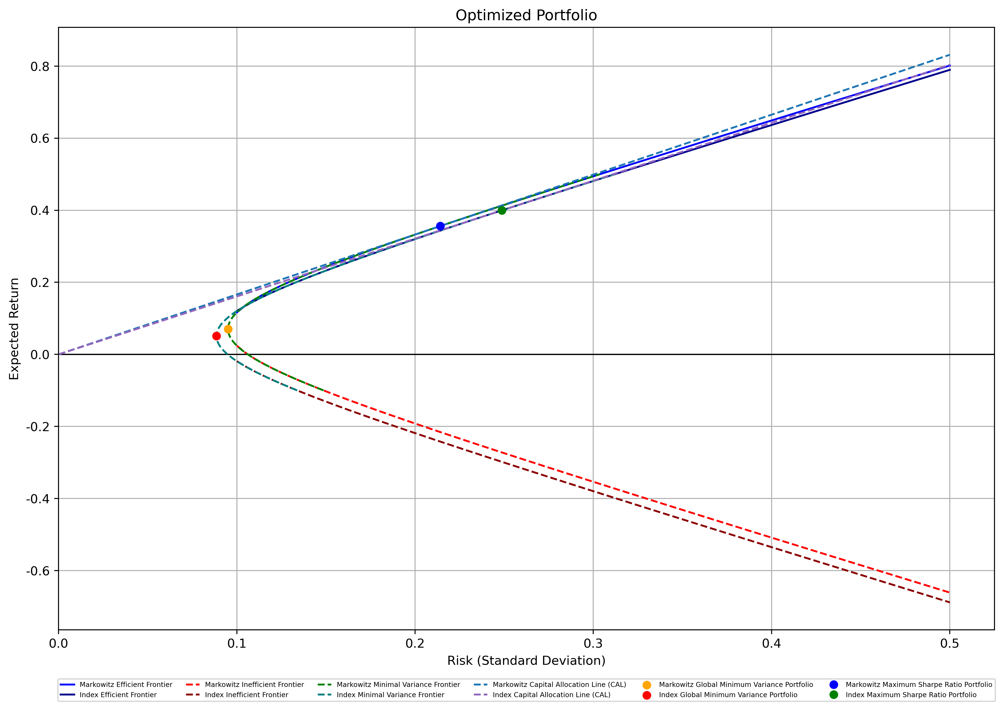
Figure 4: Minimal Variance Frontiers of Markowitz Model and Index Model Without Constraints.

3.2. Optimized Portfolios Under the First Constraint

In the second scenario, add the first constraint to the portfolio. That is, the sum of the absolute values of all weights needs to be less than or equal to 2 as it mocks Regulation T by FINRA, which states that investors are not allowed to borrow more than 50% of the purchase price from the broker-dealers. Compared to the first scenario discussed, the portfolio optimized by the Index Model generally performed better: for the Minimum Variance Portfolio, the Index Model produced a portfolio with a risk of merely 8.86%, whereas the risk of such a portfolio produced by the Markowitz Model is 9.51%; for the Max Sharpe Ratio Portfolio, the portfolio optimized by the Index Model has a Sharpe Ratio of 1.58, while the one optimized by the Markowitz Model only has a Sharpe Ratio of 1.57 (table 5 and table 6).

Table 5: Optimized Portfolio Under First Constraint Using the Markowitz Model.

Table 6: Optimized Portfolio Under First Constraint Using the Index Model.

As shown in Figure 5, the frontier lines of the Index Model look higher and to the left compared to those of the Markowitz Model. The CAL of the Index Model also has a larger slope than the CAL of the Markowitz Model, confirming the above mentioned conclusion.

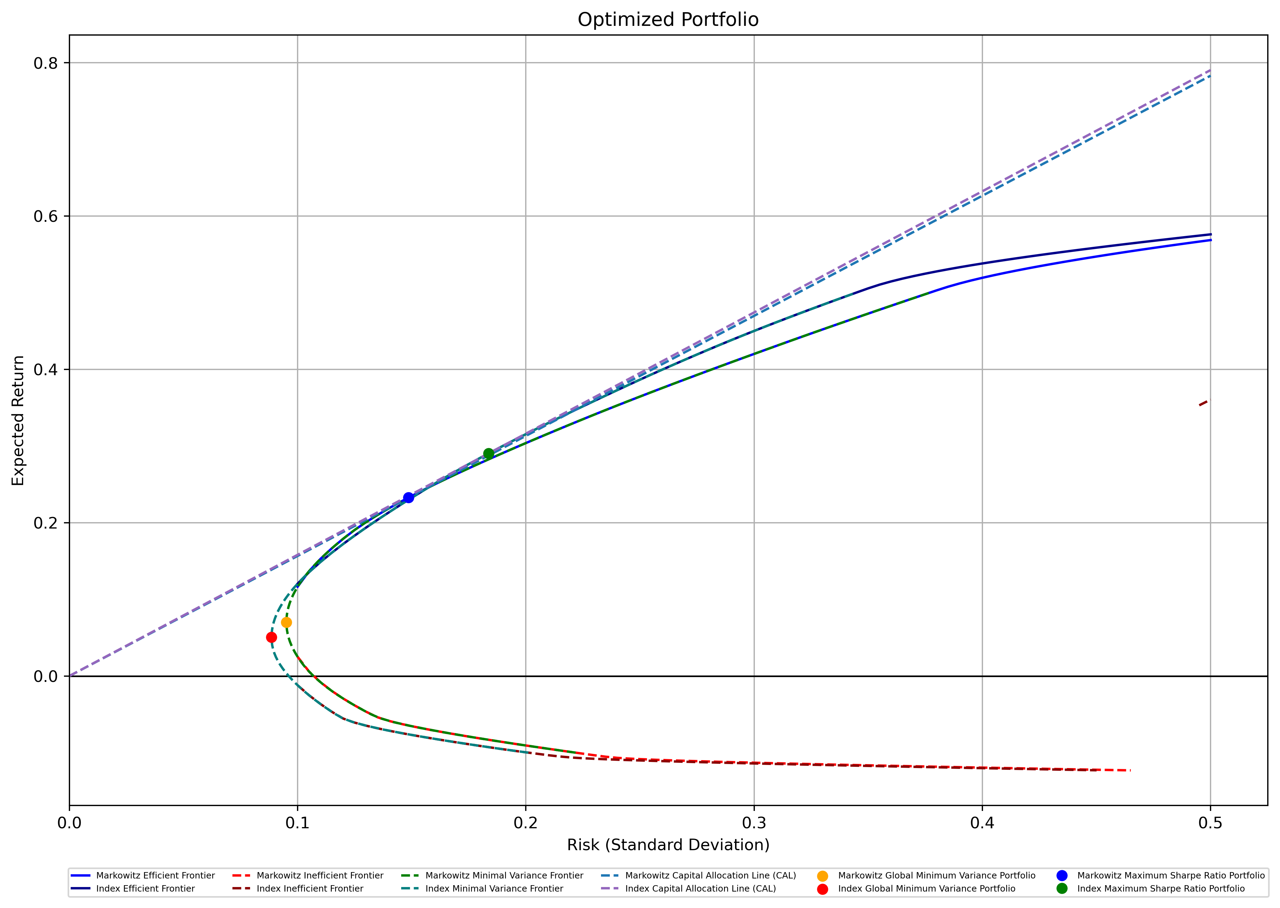
Figure 5: M-V Frontiers of Markowitz and Index Models Under the First Constraint.

3.3. Optimized Portfolios Under the Second Constraint

The second additional constraint simulates the arbitrary box constraint that allows users to set upper and lower bounds on the weights of the assets. In this case, choose an upper bound that limits the absolute value of any weight under 1.

As can be seen from Figure 6, once again, both models produced very similar results, especially the portfolios that lie on the efficient frontiers. However, under the second constraint, Markowitz performed slightly better on the efficient frontiers whereas the Minimum Variance Portfolio optimized by the Index Model has a smaller risk comparatively.

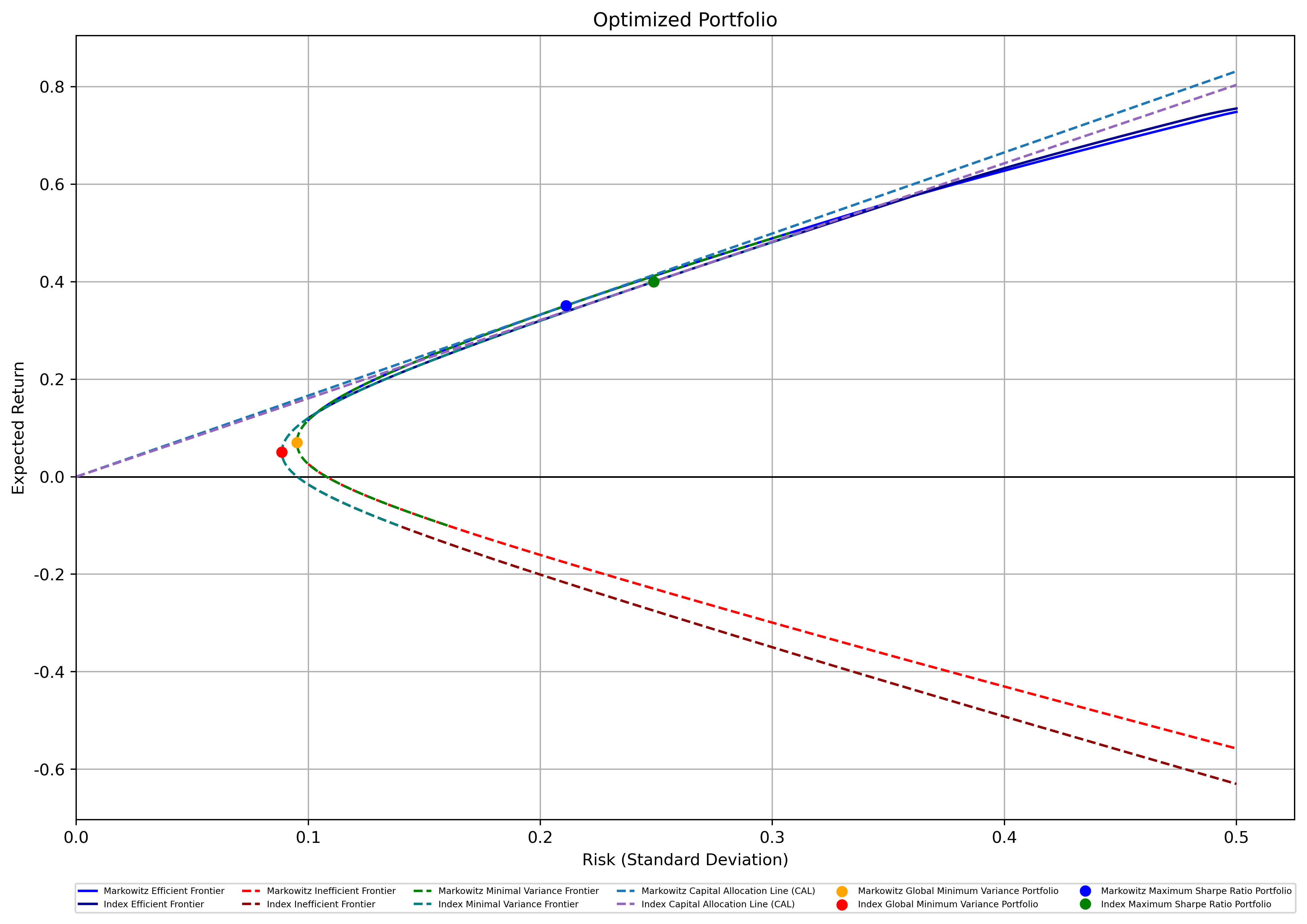
Figure 6: M-V Frontiers of Markowitz and Index Models Under the Second Constraint.

3.4. Optimized Portfolios Under the Third Constraint

The third constraint is designed to simulate the limitations in the mutual funds industry in the United States. It is stipulated that the U.S. mutual fund is not allowed to have any short positions, meaning that all weights have to be positive (table 7 and table 8).

Table 7: Optimized Portfolio Under the Third Constraint Using the Markowitz Model.

Table 8: Optimized Portfolio Under the Third Constraint Using the Index Model.

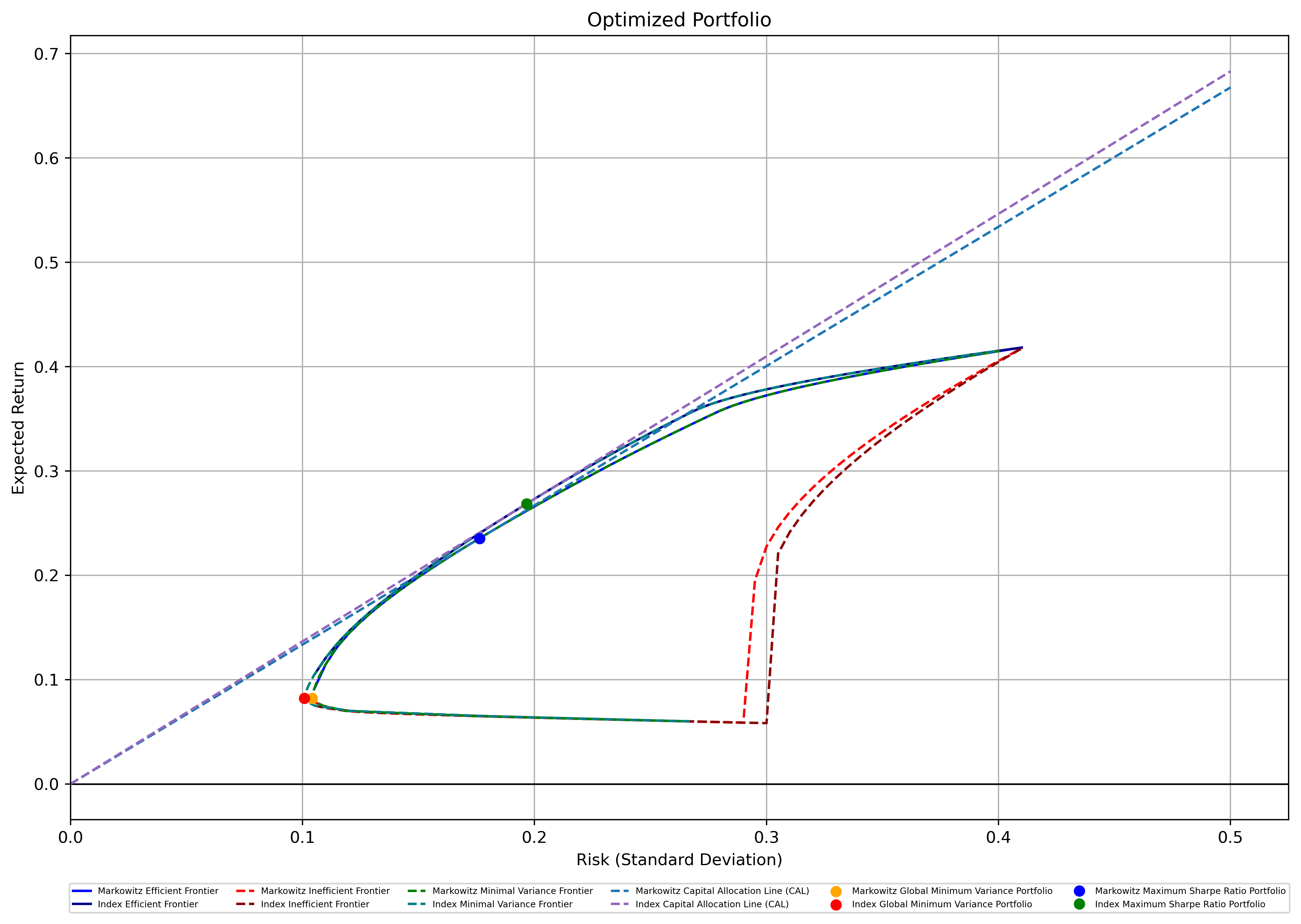
Figure 7: M-V Frontiers of Markowitz and Index Models Under the Third Constraint.

This constraint has yielded larger returns in the Minimum Variance Portfolios under both models than those under previous constraints. As can be seen from the Minimal Variance Frontiers in Figure 7, there’s no part of the frontiers that has a negative expected return. However, despite the mutual fund being considered a low-risk investment, the Sharpe ratios of both optimal portfolios under both the Markowitz Model and the Index Model are quite low. In this situation, the two models performed extremely alike, yet the Index Model has a larger Sharpe Ratio on the efficient frontiers and a steeper CAL than the Markowitz Model.

3.5. Optimized Portfolios Under the Fourth Constraint

The final constraint is designed to test the effect of the inclusion of the broad index in the portfolio. The risky portfolio is now built by ten stocks only after the weight of the S&P 500 is manually set to 0. Surprisingly, both the Markowitz Model and the Index Model produced some huge returns under this constraint. To begin with, the Minimum Variance Portfolio optimized by the Markowitz Model has a return as high as 10.14%, whereas the Max Sharpe Ratio Portfolio optimized by the Index Model possesses a return of 32.74%, which is the highest return among Max Sharpe Ratio Portfolios optimized by the two models under all conditions. However, greater gains come with larger risks. Larger standard deviations make the Sharpe ratios less appealing, and the slopes of the CALs of both models under the fourth constraint are not very different from the previous ones as can be told from Figure 8. However, under this circumstance, despite the result of the two models being very close, the Markowitz Model outperformed the Index Model with a slightly larger Sharpe Ratio of 1.61 (table 9 and table 10).

Table 9: Optimized Portfolio Under the Third Constraint Using the Markowitz Model.

Table 10: Optimized Portfolio Under the Third Constraint Using the Index Model.

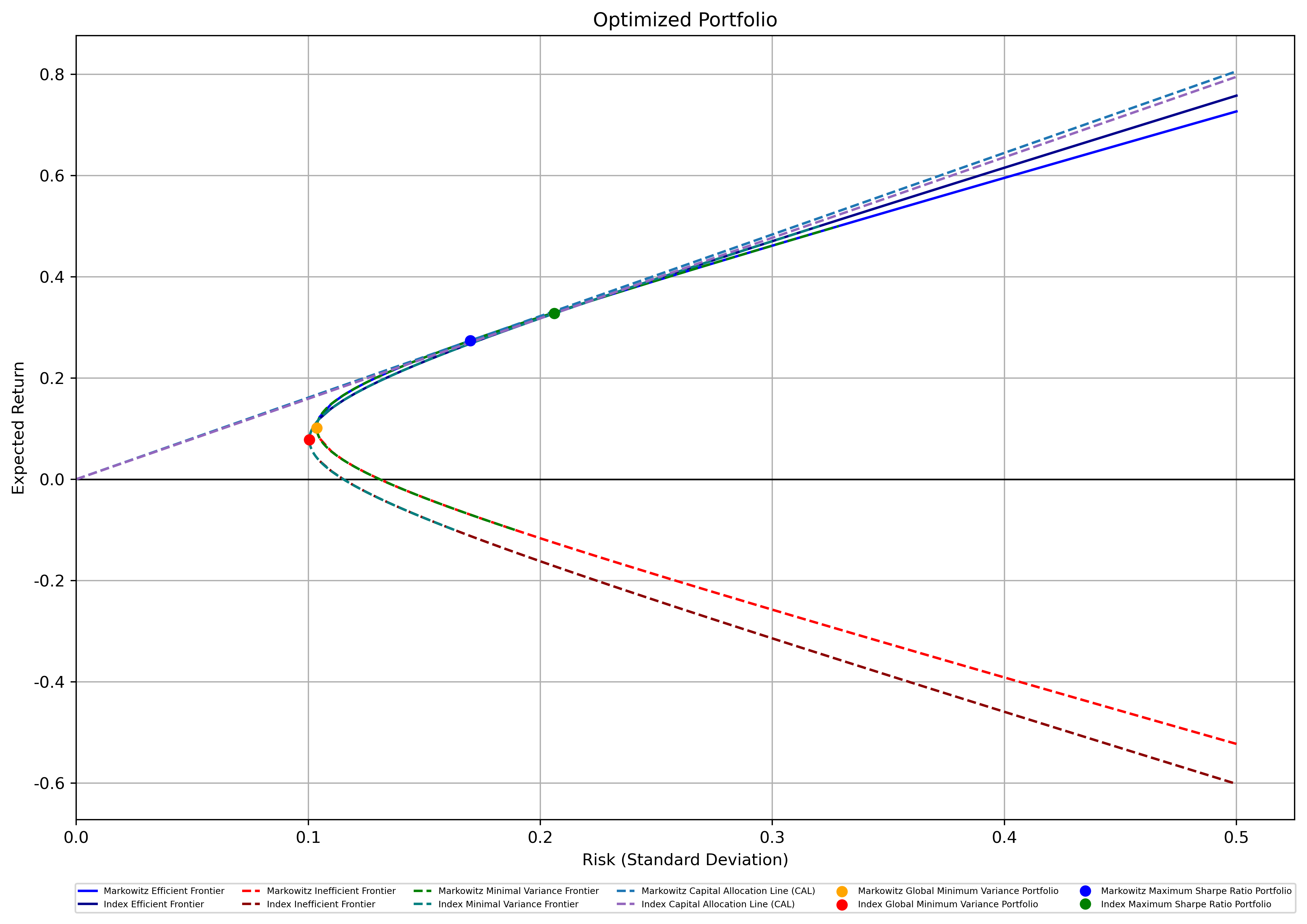
Figure 8: M-V Frontiers of the Markowitz and Index Model Under the Fourth Constraint.

4. Discussion

Finally, two Monte-Carlo simulations have been run to test the Minimal Variance Frontiers, and figure 9 demonstrates one of them. Since all the investment portfolios with different combinations simulated by the Monte-Carlo simulation are to the right and bounded by the frontiers, the models used have been proven correct and feasible. By examining the results of both the Minimum Variance Portfolio and the Maximum Sharpe Ratio under 5 different scenarios described above, it is concluded that both the Markowitz Model and the Index Model Provide correct and closely resembled results.

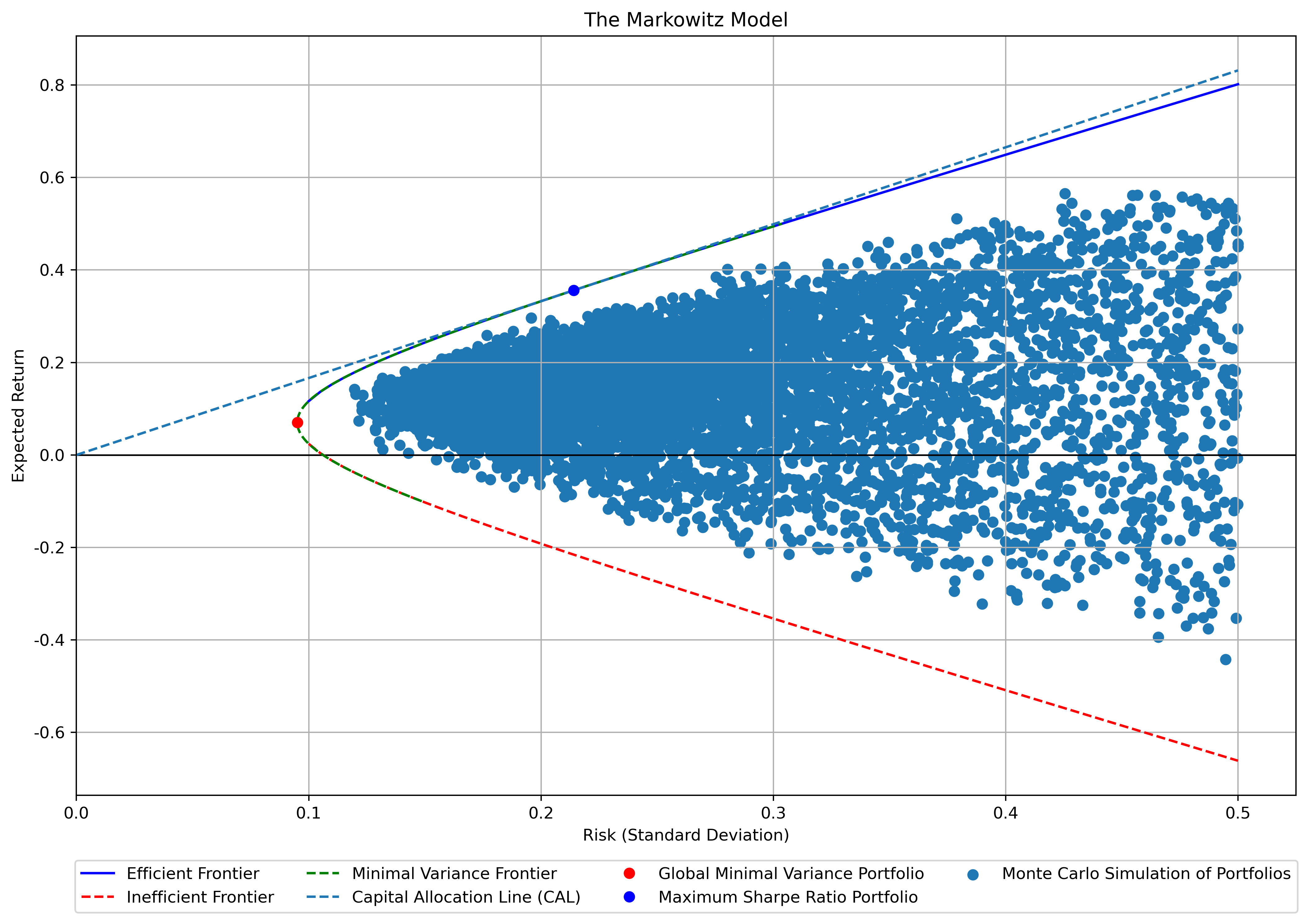
Figure 9: Monte-Carlo simulations on the Minimal Variance Frontiers

5. Conclusion

This study discusses the differences between the Markowitz Model and the Index Model under different constraints using the sample of 10 stocks in 4 sectors. It is found that both the Markowitz Model and the Index Model Provide correct and closely resembled results.

However, the Markowitz Model generally yielded a slightly more sanguine outcome with a higher Sharpe Ratio and larger return under the first scenario and additional constraints 2 and 4, while the Index model produced more auspicious outcomes under additional constraints 1 and 3. Furthermore, the Index Model is more favorable to the calculations in optimizing investment portfolios as its less optimistic result may be more realistic due to less unreliable estimates in the model-building process. After all, moderating expectations is crucial for investment.

References

[1]. Markowitz, H. (1952) Portfolio Selection. The Journal of Finance, 7(1): 77-91.
[2]. Sharpe, W. F. (1963) A Simplified Model for Portfolio Analysis. Management Science, 9(2), 277-293.
[3]. Putra, I. K. A. A. S., and Dana, I. M. (2020). Study of optimal portfolio performance comparison: Single index model and Markowitz model on LQ45 stocks in Indonesia stock exchange. American Journal of Humanities and Social Sciences Research (AJHSSR), 4(12), 237-244.
[4]. Cao, S. (2023). Comparison of Markowitz Model and Index Model in Optimization of Portfolio. Advances in Education, Humanities and Social Science Research, 5(1), 342-342.
[5]. Ni, H. (2022, April). Application and Comparison of Markowitz Model and Index Model in Hong Kong Stock Market. In 2022 7th International Conference on Social Sciences and Economic Development (ICSSED 2022) (pp. 1779-1784). Atlantis Press.
[6]. Qin, C. (2023). Comparison of Markowitz Model and Index Model for Portfolio Optimization in the Chinese Stock Market. Advances in Education, Humanities and Social Science Research, 5(1), 342.
[7]. Zhang, X. (2024). Application and Comparison of Index Model and Markowitz Model in American Stock Market. Highlights in Business, Economics and Management, 24, 808-817.
[8]. Qu, K., Tian, Y., Xu, J., and Zhang, J. (2021, December). Comparison of the Applicability of Markowitz Model and Index Model Under 5 Real-World Constraints for Diverse Investors. In 2021 3rd International Conference on Economic Management and Cultural Industry (ICEMCI 2021) (pp. 1323-1332). Atlantis Press.
Cite this article
Li,G. (2024). The Research on the Differences Between the Markowitz Model and the Index Model under Different Constraints. Advances in Economics, Management and Political Sciences,139,98-110.
Data availability
The datasets used and/or analyzed during the current study will be available from the authors upon reasonable request.
Disclaimer/Publisher's Note
The statements, opinions and data contained in all publications are solely those of the individual author(s) and contributor(s) and not of EWA Publishing and/or the editor(s). EWA Publishing and/or the editor(s) disclaim responsibility for any injury to people or property resulting from any ideas, methods, instructions or products referred to in the content.
About volume
Volume title: Proceedings of the 3rd International Conference on Financial Technology and Business Analysis
© 2024 by the author(s). Licensee EWA Publishing, Oxford, UK. This article is an open access article distributed under the terms and
conditions of the Creative Commons Attribution (CC BY) license. Authors who
publish this series agree to the following terms:
1. Authors retain copyright and grant the series right of first publication with the work simultaneously licensed under a Creative Commons
Attribution License that allows others to share the work with an acknowledgment of the work's authorship and initial publication in this
series.
2. Authors are able to enter into separate, additional contractual arrangements for the non-exclusive distribution of the series's published
version of the work (e.g., post it to an institutional repository or publish it in a book), with an acknowledgment of its initial
publication in this series.
3. Authors are permitted and encouraged to post their work online (e.g., in institutional repositories or on their website) prior to and
during the submission process, as it can lead to productive exchanges, as well as earlier and greater citation of published work (See
Open access policy for details).