1. Introduction

Housing prices are vital in the social economy. The growth of it has a direct contribution to GDP. Through the effect of industrial chain, real estate industry can also indirectly drive the development of related industries such as construction, finance, wholesale and retail, thereby further boosting overall economic growth. This indirect contribution often exceeds the direct contribution, creating a huge economic effect. Recently, with the speed of urbanization surging, the fluctuation in housing prices is closely related to the living quality of residents, and local economy. The real estate market is closely linked to the financial market. The purchase of real estate usually requires borrowing or lending, which facilitates the operation and development of financial institutions. Banks and other financial institutions provide financial support to home buyers by offering home loans, commercial loans and other services, and make profits from them. At the same time, fluctuations in the real estate market directly affect the stability and development of the financial market. Central banks can greatly improve the stability of housing markets by dynamically adjusting the interest rate with respect to mispricing in the housing market.

Empirical research underscores a multifaceted relationship between various economic factors and house price fluctuations. Lee identified credit shocks and housing supply shocks as the predominant drivers of long-term fluctuations in house prices [1]. In the context of Ireland, a historical decomposition of house price dynamics over the past thirty years reveals that both supply-side factors, such as housing stock, and demand-side factors, notably income levels, have played crucial roles [2]. Additionally, as highlighted in the Review of World Economics, increases in Foreign Direct Investment and portfolio flows contribute to rising house prices, with portfolio flows exerting a more persistent impact [3]. Furthermore, Glaeser et al. emphasized that future house price trends in China are likely to be heavily influenced by government decisions regarding new construction; if construction is sufficiently restricted, high prices may persist, though the potential for a housing market crash remains if these restrictions are not maintained [4]. Duranton and Diego conducted research and surveys in France and found that house prices and population density are also very strongly correlated, with higher population density, higher house prices. At the same time, the rise in housing prices has led to higher prices for building materials and technology [5]. Research by Truong et al. found that in Beijing, the oldest houses are concentrated in the central area, while the newest houses are in the suburbs. The most expensive houses are also concentrated in the central area, while the cheapest houses are located on the edge of the suburbs, so house prices are also affected by location [6].

This work studies influencing factors of housing price, the results can assist governments to conduct rationale housing policy, businesses to make investment strategies and individuals to make house-purchasing decisions.

2. Methods

2.1. Data Source

The dataset from “Kaggle” about the housing price in Boston is updated until 2023. There are 509 observations including multiple characteristics of houses in the Boston area for statistical analysis such as regression modeling.

2.2. Variable Selection and Description

Housing prices in Boston are governed by the dynamics of the local economy, they change according to the development of the city with significant influences from major local and regional events. Major shifts on the market come out at irregular periods and are difficult to forecast; changes in prices are frequent and hard to define in magnitude. These trends are very much conditioned by multitudes of factors, including features of neighborhoods, levels of crime, and proximity to job centers, making the Boston housing market dynamic and complex [7, 8].

The variable “MEDV” refers to the median value of owner-occupied homes in $1000's. This histogram represents the distribution of the median value of owner-occupied homes in Boston measured in thousands of dollars. The distribution is skewed towards the right; most of the homes (76) fall between $19,000 and $21,000. There is a remarkable concentration from $17,000 to $25,000, and then the number of homes drops drastically for those above $25,000 in value. As the values go higher than $27,000, the frequencies gradually get smaller, and only a very few exceed $40,000. From this histogram, it will be inferred that most of the houses are valued below $25,000 with the density in the lower to mid-value range for houses (Figure 1).

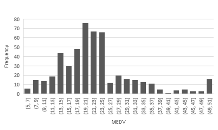
Figure 1: Histogram of MEDV.

2.3. Method Introduction

This paper encompasses the Multiple Linear Regression (MLR) model with respect to the estimation of the relation between multiple independent variables and the price of housing [9, 10]. The MLR model is comprehensive in describing how multiple different factors interplay and affect the outcome. Independent variables could be some of those factors that affect house prices, while all their coefficients are calculated by the model to measure their respective effects. Hence, the optimal fitting line would be appropriate for getting the line of best fit and obtaining the line with the least sum of squares of residuals. Hence, this method is suitable for forecasting outcomes or searching for important predictors among the huge number of possible impacts; hence, this tool is very helpful for analyzing and forecasting house prices.

\( {H_{i}}=C+{β_{1}}{x_{1}}+{β_{2}}{x_{2}}+{β_{i}}{x_{i}}+u \) (1)

3. Results and Discussion

3.1. Model Results

Through regression analysis, this paper gains several conclusions about the impact of different factors on house prices. Firstly, the coefficient of crime rate (CRIM) suggests that the median home price will drop by $114.8 for each unit increase in the crime rate, reflecting the fact that the higher crime rate makes people reluctant to buy homes in the area, leading to a drop in house prices (Table 1).

Secondly, the number of rooms (RM) will rise house prices and for each additional room, the median house price is expected to increase about $3,752.9. What’ more, the air quality also plays an important role in determining house prices, especially the nitrogen oxide concentration (NOX) which is significantly negatively correlated with house prices, and the coefficient of NOX is -18.3012, which suggests that each unit increase in NOX leads to a decrease in the median house price.

The distribution of educational resources also affects house prices [10]. The study finds that the pupil-teacher ratio (PTRATIO) is negatively correlated with house prices, with a regression coefficient of -0.9677. This indicates that for each unit increase in the pupil-teacher ratio, the median house price will decrease by $967.7.

Additionally, factors such as the property tax rate (TAX), distance to employment centers (DIS), and highway accessibility (RAD) also have some influence on house prices. Higher property tax rates are associated with lower house prices, homes farther away from employment centers tend to be less expensive and better highway accessibility correlates with higher prices.

Table 1: Model results.

3.2. Multicollinearity Check

From the VIF analysis, there is a strong multicollinearity in tax's VIF value of 9.12, which is close to the critical value of 10, indicating that this paper needs to pay special attention, but not to a very serious extent (Table 2).

Table 2: VIF results.

The VIF value of 7.54 for rad shows slightly higher multicollinearity and needs to be concerned. nox, indus and dis have moderate VIF values of 4.37,4.00and 3.99 respectively and their data suggests that they have a multicollinearity problem but not serious.

The values of age and lstat show moderate covariance with 3.09 and 2.92 respectively, which shows that they have moderate covariance, but the effect is less. The VIF value of zn is 2.32, indicating a mild problem of covariance. Then the VIF values of rm, ptratio and crim are 1.95,1.82and 1.82 respectively, again showing a very low impact. The remaining b and chas have VIF values of 1.35 and 1.07 respectively, showing that they are hardly affected.

3.3. Homoscedasticity Test

Heteroscedasticity, which refers to the fact that in a regression model, the variance of the error term is not constant, but changes as the independent variable changes. This property violates an important assumption of classical linear regression models, that is, the homoscedasticity hypothesis, which guarantees that the regression parameter estimators have good statistical properties. Therefore, if the model is heteroscedasticity, statistical inferences based on the assumption of the homoscedasticity hypothesis may be affected, resulting in biased or inconsistent estimates. In regression analysis, heteroscedasticity refers to the unequal scatter of residuals or error terms. Specifically, it refers to the case where there is a systematic change in the spread of the residuals over the range of measured values (Figure 2).

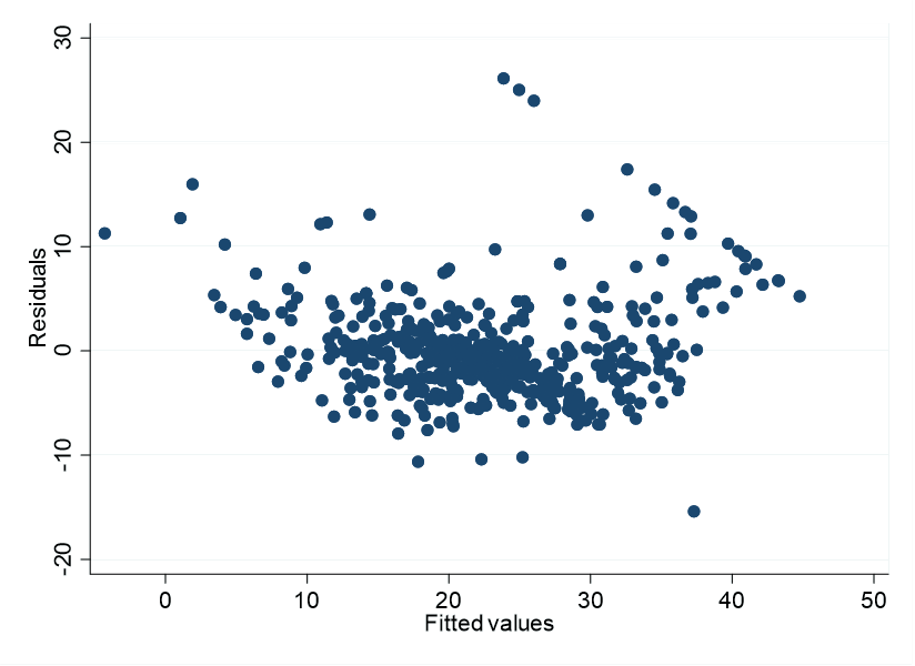
Figure 2: Scatter diagram of residuals.

The author draws the residuals to observe the trend of residuals and judge whether there is heteroscedasticity. This image presents a scatter plot of residuals versus fitted values and the residual is the difference between the observed value and the predicted value by the model.

In the graph, each point represents an observation, with the x-axis denoting the fitted values and the y-axis showing the residuals. Visually, these points appear to be randomly dispersed without any noticeable trend or pattern. This suggests that in this dataset, the residuals do not systematically increase or decrease as the fitted values change. Additionally, most points cluster around the central region of the coordinate system, indicating that most residuals are relatively small and evenly distributed around zero. However, there are also some larger residuals present, which deviate further from the zero line. These large residuals may suggest poor adaptation of certain sample points to the model or the presence of outliers. There is no obvious aggregation phenomenon or significant increase or decrease of residuals, so there's no heteroscedasticity problem.

In the study, this paper analyzed the impact of different factors affecting house prices in the Boston area, such as crime rates, air quality, and other variables on house prices, mainly using multiple linear regression models. In contrast to previous studies, Qi also used multiple regression analysis to analyze housing prices in Chongqing, but his study focused on the southwest region of China, which was then applied to the development of more rational real estate policies [7]. There is also an article that focuses on the key factors affecting housing renovations (e.g., renovations, extensions, etc.) and home pricing, and this study uses the Hedonic Pricing Model (HPM) to analyze how a variety of environmental and architectural characteristics affect home prices, and ultimately it concludes that environmental factors are the most influential in terms of home prices [8].

4. Conclusion

Overall, Boston housing prices depend quite strongly on various factors, among which are rates of crime, air quality, and travel-to-work, as introduced above. The findings emphasize that the housing market is very complicated, where local economic development and neighborhood features play a pivotal role in price variation. This insight is valuable for policymakers, real estate investors, and future homeowners in their regard, as it helps them make well-considered decisions. However, such findings are relevant to stakeholders concerned with the wider implications for economic growth and financial stability, emphasizing that it is critical to ensuring a balanced, thriving housing market. Housing price dynamics are reflections and key determinant of economic health, hence an important subject in economic planning and development strategies.

Authors Contribution

All the authors contributed equally and their names were listed in alphabetical order.

References

[1]. Lee, J. (2024) What factors drive house prices in the USA. Empire Econ, 66, 2533-2556.
[2]. Paul, E., et al. (2024) How supply and demand affect national house prices: The case of Ireland. Journal of Housing Economics, 65, 1051-1377.
[3]. Hernandez, V.M. (2023) How relevant are capital flows for house prices in emerging economies? Rev World Econ, 159, 965-986.
[4]. Glaeser, E. et al. (2017) A Real Estate Boom with Chinese Characteristics. The Journal of Economic Perspectives, 31, 93-116.
[5]. Duranton, G. and Diego, P. (2020) The Economics of Urban Density. The Journal of Economic Perspectives, 34.
[6]. Truong, Q., et al. (2020) Housing price prediction via improved machine learning techniques. Procedia Computer Science, 174, 433-442.
[7]. Qi, Y. (2024) Research on the Influencing Factors of Housing Prices Based on Multiple Regression: Taking Chongqing as an Example. Applied Economics and Policy Studies. Springer, Singapore.
[8]. Portnov, B.A., Odish, Y. and Fleishman, L. (2005) Factors Affecting Housing Modifications and Housing Pricing: A Case Study of Four Residential Neighborhoods in Haifa, Israel. The Journal of Real Estate Research, 27(4), 371-408.
[9]. Uyanık, G.K. and Neşe, G. (2013) A study on multiple linear regression analysis. Procedia-Social and Behavioral Sciences, 106, 234-240.
[10]. Zhang, J.K., et al. (2020) Meta-analysis of the relationship between high quality basic education resources and housing prices. Land Use Policy, 99, 104843.
Cite this article
Du,K.;Li,Y.;Liu,R. (2025). The Research on Influencing Factors of Housing Price. Advances in Economics, Management and Political Sciences,155,1-6.
Data availability
The datasets used and/or analyzed during the current study will be available from the authors upon reasonable request.
Disclaimer/Publisher's Note
The statements, opinions and data contained in all publications are solely those of the individual author(s) and contributor(s) and not of EWA Publishing and/or the editor(s). EWA Publishing and/or the editor(s) disclaim responsibility for any injury to people or property resulting from any ideas, methods, instructions or products referred to in the content.
About volume
Volume title: Proceedings of the 3rd International Conference on Financial Technology and Business Analysis
© 2024 by the author(s). Licensee EWA Publishing, Oxford, UK. This article is an open access article distributed under the terms and
conditions of the Creative Commons Attribution (CC BY) license. Authors who
publish this series agree to the following terms:
1. Authors retain copyright and grant the series right of first publication with the work simultaneously licensed under a Creative Commons
Attribution License that allows others to share the work with an acknowledgment of the work's authorship and initial publication in this
series.
2. Authors are able to enter into separate, additional contractual arrangements for the non-exclusive distribution of the series's published
version of the work (e.g., post it to an institutional repository or publish it in a book), with an acknowledgment of its initial
publication in this series.
3. Authors are permitted and encouraged to post their work online (e.g., in institutional repositories or on their website) prior to and
during the submission process, as it can lead to productive exchanges, as well as earlier and greater citation of published work (See
Open access policy for details).