1. Introduction

Risk management is a crucial element of quantitative finance, offering a framework for evaluating and alleviating potential losses in investment portfolios [1]. This study focuses on how to construct portfolios that balance risk and return. The objective is to estimate the 99% and 95% VaR for a portfolio composed of the S&P 500, representing the United States, and the DAX, representing Europe.

Volatility, central to risk estimation, is modeled using time-series techniques such as GARCH. Nevertheless, stock prices exhibit time-dependent behavior, where historical patterns impact future movements, which makes such models particularly suited for this analysis [2]. Moreover, Monte Carlo simulations further expand this framework by generating scenarios that incorporate these dynamics to assess portfolio risk.

The methodology begins by transforming the indices’ price data into log returns to standardize the analysis. Then, AR models are used to capture mean dynamics, while GARCH models address volatility clustering. Residuals from these models are transformed using the Probability Integral Transform (PIT) to achieve uniformity. The dependency structure is modeled using a Copula function, which links the indices' marginal distributions. Simulated errors are transformed back to scaled residuals, which are used to calculate portfolio returns.

This research aims to quantify the risk associated with a geographically diversified portfolio and evaluate Monte Carlo simulation as a robust method for VaR estimation.

2. Data Collection

The main purpose of this study is to construct an investment portfolio consisting of two selected stock indices and calculate their Value at Risk (VaR) at 99% and 95% confidence levels. Therefore, this article examines the correlation between two prominent stock indices representing distinct economic regions: the S&P 500 (U.S. market index) and the DAX (European market index).

The data used in this article covers weekly closing price data from 2000 to 2023, sourced from Yahoo Finance. This long-time span data can not only reflect the long-term dynamic characteristics of the two indexes, but also capture the impact of important historical market events on yields and volatility, such as the global financial crisis in 2008 and the impact of the COVID-19 pandemic in 2020.

3. Methodology

The methodology of this study involves several key steps to estimate the Value at Risk (VaR) of a geographically diversified portfolio. First, data preprocessing is performed by calculating log returns to normalize price data and ensure its suitability for modeling. Missing values and outliers are removed to maintain data quality. The formula for log returns is:

\( {r_{t}}=ln{({P_{t}})}-ln⁡({P_{t-1}}) \) (1)

Next, the stationarity of the log returns is tested using the Augmented Dickey-Fuller (ADF) test, which helps confirm the data's stability for time series analysis [3]. This is followed by an autoregressive (AR) model applied to capture the autocorrelation in returns, with the model order chosen based on the Akaike Information Criterion (AIC) and Bayesian Information Criterion (BIC) for optimal fit. The AR model is:

\( {X_{t}}=c+\sum _{i=1}^{p}{ϕ_{i}}{X_{t-i}}+{ε_{t}} \) (2)

To model volatility, a Generalized Autoregressive Conditional Heteroskedasticity (GARCH) model is used, which accounts for volatility clustering and heavy tails in financial time series. The fundamental equations of the GARCH model are as follows:

\( {R_{t}}=μ+{ε_{t}}, σ_{t}^{2}=α+\sum _{i=1}^{p}{β_{i}}ε_{t-1}^{2}+\sum _{j=1}^{p}{γ_{j}}σ_{t-j}^{2} \) (3)

Residual diagnostics are then conducted using the Probability Integral Transform (PIT) to ensure that the residuals follow a uniform distribution, confirming the validity of the model's assumptions.

The nest step is to verify the distributional assumptions of the residuals, the probability integral transform (PIT) is applied. PIT maps residuals into the interval [0,1] using their cumulative distribution function (CDF):

\( {u_{t}}={F_{ε}}({ε_{t}}) \) (4)

where \( {u_{t}} \) should follow a uniform distribution \( U(0,1) \) if the model's distributional assumptions are correct [4].

The relationship between the returns of different indices is modeled using copulas, which capture the dependency structure between variables. Finally, Monte Carlo simulation is employed to estimate VaR by simulating multiple portfolio return paths and calculating the appropriate quantile of the distribution. The formula for VaR is:

\( Pr{(ΔP≤VaR)}=α \) (5)

4. Results

4.1. Stationarity and Autocorrelation Tests

The stationarity of SP500 and DAX log returns was assessed using the ADF test. With p-values of 0.01 for both indices, the null hypothesis of a unit root was rejected at the 5% significance level.

Autocorrelation was analyzed through the Ljung-Box test, yielding p-values of 0.035 for SP500 and 0.015 for DAX log returns. The null hypothesis of no significant autocorrelation could be rejected.

4.2. ACF and PACF Analysis

For SP500 log returns, as Figure 1 shows, the ACF plot did not display a distinct exponential decay pattern, while the PACF plot showed a significant spike at lag 1. Therefore, an AR(1) component should be included. Moreover, the ACF of squared log returns revealed strong volatility clustering.

Similarly, for DAX log returns, as Figure 2 shows, the ACF plot lacked an exponential decay pattern, while the PACF plot exhibited a prominent spike at lag 3, pointing to a potential AR(3) component. The ACF of squared returns also revealed volatility clustering.

In a nutshell, we use AR(1)-GARCH and AR(3)-GARCH models for SP500 and DAX log returns, respectively.

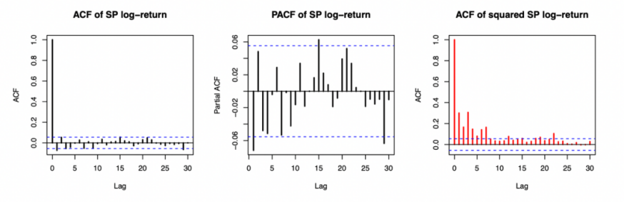
Figure 1: ACF and PCF of SP

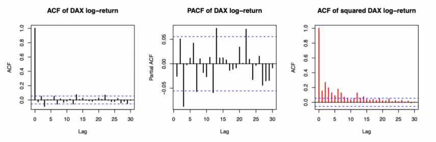
Figure 2: ACF and PCF of DAX

4.3. GARCH Model Development and Optimization

The GARCH model extends the ARCH model by incorporating longer memory effects in the conditional variance [5]. For SP500, various conditional error distributions were tested under the GARCH(1,1) framework, including normal, skew-normal, t-distribution, generalized error distribution (GED), and their skewed variants. However, none passed the Anderson-Darling (AD) and Kolmogorov-Smirnov (KS) tests for uniformity of PIT-transformed residuals. This indicates the inability of GARCH(1,1) to fully capture the asymmetric volatility and tail behavior of SP500 returns.

Given the historical asymmetric volatility patterns observed during periods 2008 financial crisis and the 2020 pandemic, a TGARCH(1,1) model was implemented. This model exhibited superior performance across all error distributions. Among these, the skewed t-distribution demonstrated the best results, with lower AIC and BIC values and higher p-values in AD and KS tests. Although its p-value in the Ljung-Box test was not the highest, it was sufficient to confirm the independence of residuals. The skewed t-distribution effectively captured the heavy tails and skewness, making it the preferred choice for the SP500 TGARCH(1,1) model.

For DAX, a similar analysis revealed that GARCH(1,1) failed to adequately model the series. TGARCH(1,1) combined with the skewed t-distribution yielded the best performance, achieving lower information criteria values and higher p-values in uniformity and independence tests. Nevertheless, the distribution’s tail properties aligned well with historical market crises, supporting its selection for modeling DAX returns. Table 1 shows the results of the two chosen distributions under TGARCH(1,1) model.

Table 1: TGARCH(1,1) test result

4.4. Incorporating Copula Functions

The concept of Copula functions originates from Sklar’s theorem [6]. This theorem establishes that for the joint cumulative distribution function \( H({x_{1}},{x_{2}}) \) of random variables \( ({x_{1}},{x_{2}}) \) , if their marginal cumulative distribution functions \( {F_{1}} \) and \( {F_{2}} \) are known, there exists a Copula function \( C \) that connects them, expressed as:

\( H({x_{1}},{x_{2}})=C({F_{1}}({x_{1}}), {F_{2}}({x_{2}}) \) (6)

For a random variable \( x \) with a distribution function \( F(x) \) , if the inverse \( {F^{-1}} \) exists, then the transformed variable \( U=F(x) \) follows a uniform distribution on [0,1].

To analyze the dependence structure between SP and DAX returns, a copula function is employed. First, PIT transforms the standardized residuals from the AR-GARCH model into uniform margins, using the formula mentioned before:

\( {u_{t}}={F_{ε}}({x_{t}}) \) (7)

The fitted copula is used to generate pseudo-random samples \( (u,v) \) in the [0,1] space [7].

After fitting TGARCH models for SP500 and DAX, a copula approach was employed to model the dependency structure of PIT-transformed residuals, see Figure 3&4. The Student-t copula was chosen based on AIC criteria, capturing the tail dependencies and joint extreme movements.

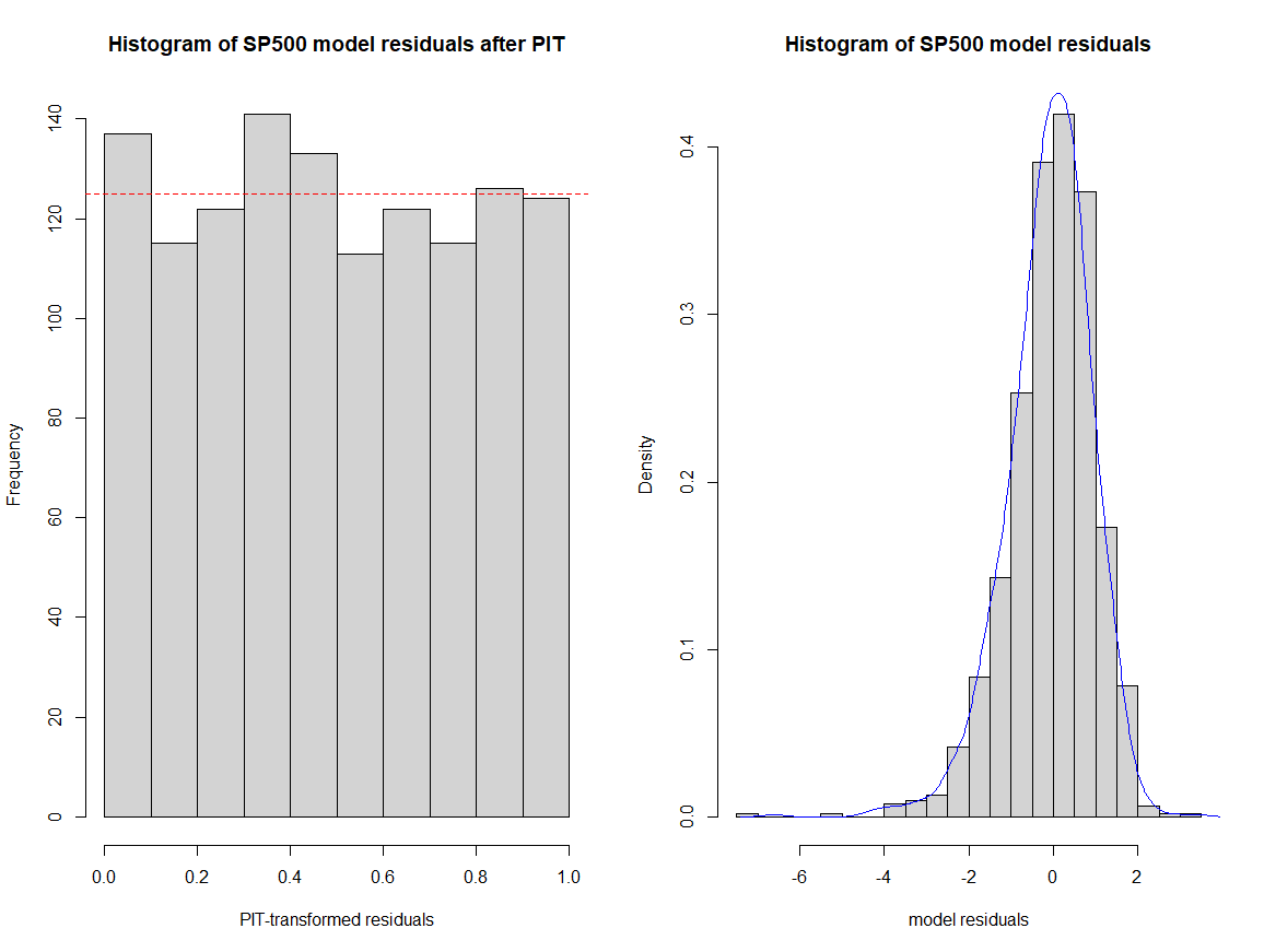
Figure 3: SP PIT Results

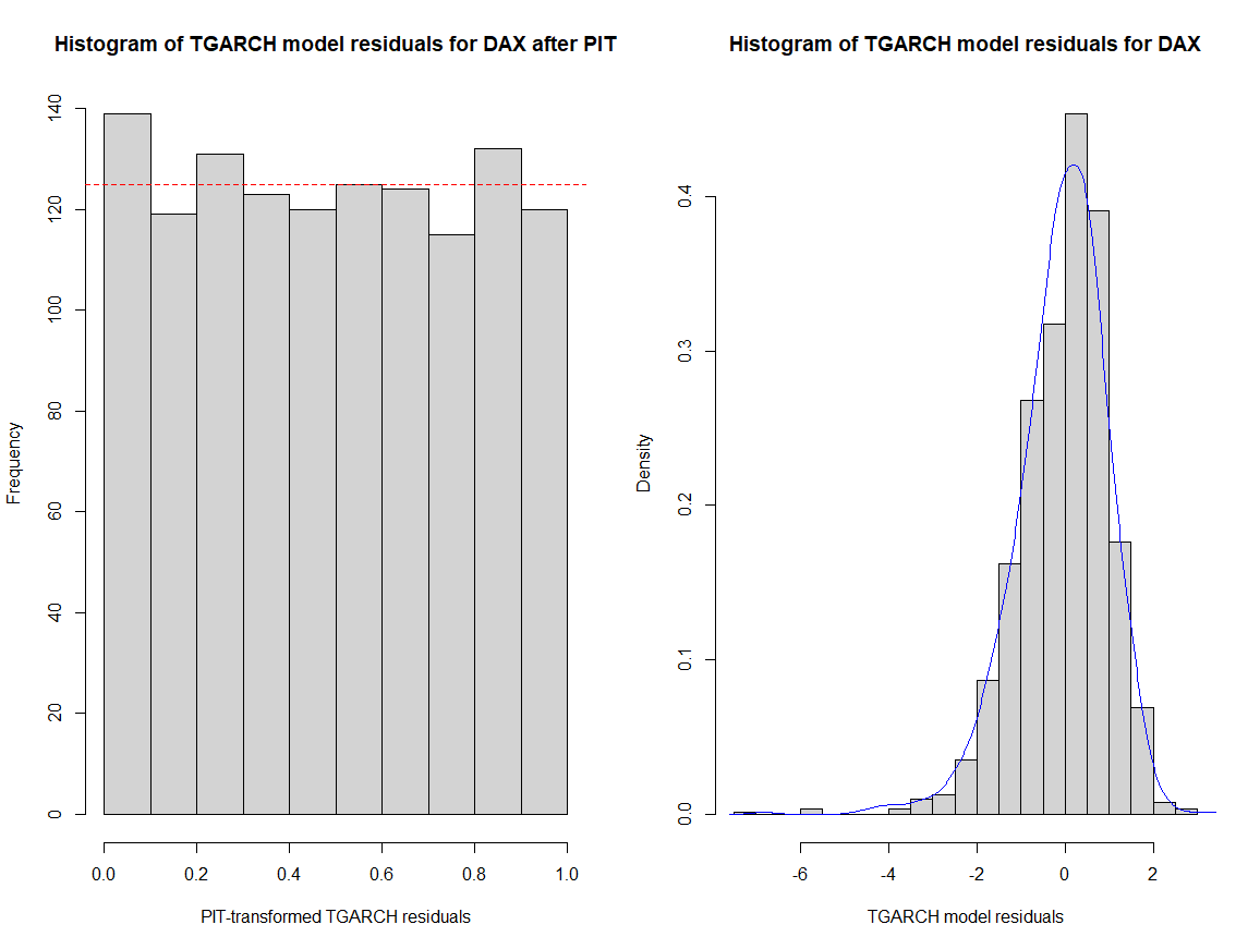
Figure 4: DAX PIT Results

4.5. VaR Estimation

Monte Carlo simulation using the AR-TGARCH model generated portfolio log returns as follows:

\( {r_{portfolio,t}}=log{(1+\frac{1}{2}({e^{{r^{sp,t}}-1}})+\frac{1}{2}({e^{{r^{DAX,t}}-1}}) )} \) (8)

By generating multiple simulated paths of portfolio returns, the conditional variance \( {σ^{2}} \) and returns \( {r_{t}} \) are computed iteratively using the AR-GARCH model [8].

The simulated log returns were analyzed to compute the 1% and 5% VaR. The 99% VaR was -0.071813, which shows a 99% probability that the weekly portfolio logarithmic loss would not exceed 7.18%. The 95% VaR was -0.035805, which implies a 95% probability that losses would not exceed 3.58%.

4.6. The Significance of Geographical Diversification

Following the same procedures, we can get the VaR of an equal weight portfolio of no geographical diversification. Here, General Electric (GE) and Microsoft (MSFT) are chosen for comparison. Both of them are American stocks.

Table 2: VaR of Different Portfolios

As Table 2 shows, at the 95% confidence level, the absolute value of VaR of the geographically diversified portfolio (SP and DAX) is slightly lower than the non-diversified portfolio (GE and MSFT). Moreover, at the 99% confidence level, the VaR of the diversified portfolio is notably lower.

This demonstrates that geographical diversification can effectively mitigate risk, which reduces the potential losses of a portfolio in extreme scenarios with no doubt. Specifically, geographical diversification reduces the impact of market or industry fluctuations on the overall portfolio by introducing assets from different regions. As a result, portfolios with geographical diversification tend to exhibit lower extreme risk when faced with uncertain market conditions.

5. Conclusion

This study evaluated the VaR of a portfolio comprising the S&P 500 and DAX indices, and estimates the 99% and 95% VaR levels using AR-TGARCH models combined with skewed Student-t distributions and a Student-t copula. The 99% VaR was calculated as -0.071813, while the 95% VaR was -0.035805. The results demonstrate that the chosen models successfully accounted for heavy tails, volatility clustering, and asymmetric effects.

For future researchers, this study suggests exploring other copula functions, such as vine copulas, to model complex dependencies in higher-dimensional portfolios [9, 10]. Machine learning algorithm models can also be introduced to evaluate and predict the volatility risk.

From a policy perspective, these findings suggest that financial regulators and institutional investors should prioritize models capable of capturing extreme market conditions. Stress-testing frameworks need to incorporate approaches such as Monte Carlo simulation with time-series and copula models. Moreover, policymakers could encourage transparency and better risk management practices by requiring institutions to report stress-tested VaR estimates at multiple confidence levels. Financial security is an important foundation for the stable and healthy development of the economy. Strengthening and improving modern financial regulation, enhancing the financial stability guarantee system, can continuously strengthen the ability to prevent and control financial risks.

References

[1]. Power, M. (2004). The risk management of everything. The Journal of Risk Finance, 5(3), 58-65.
[2]. Kim, D., & Kon, S. J. (1999). Structural change and time dependence in models of stock returns. Journal of Empirical Finance, 6(3), 283-308.
[3]. Paparoditis, E., & Politis, D. N. (2018). The asymptotic size and power of the augmented Dickey–Fuller test for a unit root. Econometric Reviews, 37(9), 955-973.
[4]. Yun, J. (2020). Density forecast evaluations via a simulation-based dynamic probability integral transformation. Journal of Financial Econometrics, 18(1), 24-58.
[5]. Lee, S. W., & Hansen, B. E. (1994). Asymptotic theory for the GARCH (1, 1) quasi-maximum likelihood estimator. Econometric theory, 10(1), 29-52.
[6]. Abe Sklar (1973). Random variables, joint distribution functions, and copulas. Kybernetika, Vol. 9, No. 6, 449—460
[7]. Lin, T., Wang, C. W., & Tsai, C. C. L. (2015). Age-specific copula-AR-GARCH mortality models. Insurance: Mathematics and Economics, 61, 110-124.
[8]. Suhobokov, A. (2007). Application of Monte Carlo simulation methods in risk management. Journal of Business Economics and Management, 8(3), 165-168.
[9]. Czado, C., Bax, K., Sahin, Ö., Nagler, T., Min, A., & Paterlini, S. (2022). Vine copula based dependence modeling in sustainable finance. The Journal of Finance and Data Science, 8, 309-330.
[10]. Dissmann, J., Brechmann, E. C., Czado, C., & Kurowicka, D. (2013). Selecting and estimating regular vine copulae and application to financial returns. Computational Statistics & Data Analysis, 59, 52-69.
Cite this article
Li,L. (2025). Risk Exposure – A Case Study of Monte Carlo Simulation. Advances in Economics, Management and Political Sciences,167,122-127.
Data availability
The datasets used and/or analyzed during the current study will be available from the authors upon reasonable request.
Disclaimer/Publisher's Note
The statements, opinions and data contained in all publications are solely those of the individual author(s) and contributor(s) and not of EWA Publishing and/or the editor(s). EWA Publishing and/or the editor(s) disclaim responsibility for any injury to people or property resulting from any ideas, methods, instructions or products referred to in the content.
About volume
Volume title: Proceedings of the 4th International Conference on Business and Policy Studies
© 2024 by the author(s). Licensee EWA Publishing, Oxford, UK. This article is an open access article distributed under the terms and
conditions of the Creative Commons Attribution (CC BY) license. Authors who
publish this series agree to the following terms:
1. Authors retain copyright and grant the series right of first publication with the work simultaneously licensed under a Creative Commons
Attribution License that allows others to share the work with an acknowledgment of the work's authorship and initial publication in this
series.
2. Authors are able to enter into separate, additional contractual arrangements for the non-exclusive distribution of the series's published
version of the work (e.g., post it to an institutional repository or publish it in a book), with an acknowledgment of its initial
publication in this series.
3. Authors are permitted and encouraged to post their work online (e.g., in institutional repositories or on their website) prior to and
during the submission process, as it can lead to productive exchanges, as well as earlier and greater citation of published work (See
Open access policy for details).