1. Introduction

Investment portfolio construction is a critical topic in quantitative finance. Effective portfolio construction can significantly impact an investor's success, making it a key area of focus for financial researchers and practitioners.

The construction of an investment portfolio can be divided into two primary steps: asset selection and asset allocation. The first step is to select the specific assets that will the portfolio. This involves filtering and choosing high-quality assets that align with the investor's goals and risk tolerance. The next step involves determining the proportion of the total portfolio to allocate to different asset classes or individual assets. Various methods can be employed, including the use of optimization models and heuristic approaches.

One of the foundational methods for asset allocation is the mean-variance model introduced by Markowitz. This model provides a framework for constructing an optimal portfolio by balancing expected returns against the volatility of those returns. The mean-variance model assumes that investors are rational, seeking to maximize returns for a given level of risk.

Effective portfolio construction requires the identification of high-quality assets, which is often achieved through pre-selection processes. These processes typically involve forecasting stock market performance to identify assets with high potential returns.

Traditionally, stock prediction has relied on various statistical and econometric methods, such as time series analysis and regression models. However, with advancements in technology and data availability, machine learning have emerged as powerful tools for stock market prediction. These methods can capture complex patterns and interactions in financial data that traditional methods might miss. One prominent method in machine learning is the Long Short-Term Memory (LSTM) neural network. LSTM excels in time series prediction because it can retain long-term dependencies and patterns within data, making it a valuable tool for forecasting stock prices and recognizing potential investment opportunities.

This paper aims to address the two key steps in investment portfolio construction: stock pre-selection and mean-variance model construction. First, a method to pre-select stocks based on their predicted performance using LSTM will be implemented. Second, a portfolio will be constructed using the mean-variance model with the pre-selected stocks. Finally, the performance of the constructed portfolios will be evaluated using a series of metrics to compare their effectiveness. This comprehensive approach combines modern machine learning techniques with classical financial models to enhance portfolio construction strategies.

2. Related work

The Efficient Market Hypothesis (EMH) [1] and the Random Walk Hypothesis (RWH) [2] have long suggested that stock price movements are largely unpredictable. According to these hypotheses, all available information is already reflected in stock prices, and any future price changes are the result of new information, which by definition is random and unpredictable. However, recent research has challenged this view, suggesting that stock prices can, to some extent, be predicted [3].

Several authors have proposed various methodologies for predicting stock prices. The mainstream approaches can be broadly categorized into statistical methods and machine learning methods. Statistical methods, such as ARCH [4], GARCH [5] and ARIMA [6], have been widely used for time series analysis and forecasting in financial markets. These models are valued for their ability to model volatility clustering and trends within time series data. Machine learning methods, including Support Vector Machines (SVM) [7] and Random Forest [8], have also been applied to stock price prediction with notable success. These methods can capture complex, non-linear relationships within data that traditional statistical methods may miss.

With the development of deep learning, there has been a significant shift towards using more sophisticated models for stock prediction. Deep learning models, particularly Long Short-Term Memory (LSTM) networks, have shown promise in handling the intricacies of stock market data. LSTM, a variant of Recurrent Neural Networks (RNN), addresses some of the key limitations of traditional RNN models, such as the vanishing gradient problem and difficulty in managing long sequences of data. Hochreiter and Schmidhuber (1997) introduced LSTM networks [9], which use carefully designed hidden layer neurons to mitigate the gradient vanishing issue. By maintaining long-term dependencies and patterns within the data, LSTM networks are better suited for time series prediction tasks like stock price forecasting.

As deep learning continues to evolve, more researchers such as [10,11] are exploring its potential in financial applications. The flexibility and power of LSTM networks make them a popular choice for modeling the dynamic and complex nature of stock markets, pushing the boundaries of what is considered predictable in the realm of finance.

3. Methodology

3.1. LSTM neural networks

Traditional RNNs are designed to pass information across time steps through hidden layers, allowing for sequential data processing. However, they often struggle with long-term dependencies due to issues like vanishing and exploding gradients, making it difficult to capture patterns in long sequences.

LSTM networks overcome these challenges by introducing three key gates: the input gate, forget gate, and output gate. These gates work together to manage the flow of information, enabling LSTMs to selectively retain or discard data over time. The forget gate decides which information from the previous cell state should be forgotten, the input gate determines which new information should be added, and the output gate controls the next hidden state based on the current cell state. This gating mechanism allows LSTMs to handle long-term dependencies effectively, making them particularly useful for tasks such as time series prediction. In this study, the LSTM model utilizes historical stock return data along with technical indicators to predict future returns, leveraging its strength in learning from long-term patterns in data.

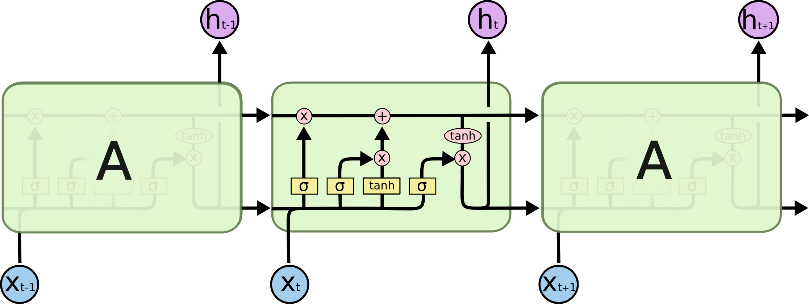
Figure 1: LSTM memory cell structure

3.2. Mean-variance model

The mean-variance model, grounded in the assumption of rational investor behavior, aims to either maximize expected return for a given level of risk or minimize risk for a desired return. This model identifies the efficient frontier, which represents the optimal trade-off between risk and return across all possible portfolios. The core advantage of the Markowitz approach is its provision of an explicit analytic solution, allowing for a detailed analysis of portfolio characteristics. The expected return of a portfolio is calculated as the weighted sum of the expected returns of individual assets, while the portfolio's risk is determined by the variance of returns, which accounts for covariances between assets.

In our study, we first rank the stock returns predicted by the LSTM model, using the expected return as the criterion for selecting "high quality assets." Subsequently, the selected stocks are utilized to construct the investment portfolio employing the mean-variance model.

4. Experiment and results

4.1. Data

We selected 20 constituent stocks from the FTSE 100 index on Yahoo Finance as our sample data. The data selected are at daily frequency. To capture the long-term patterns of stock movements, we chose a time span from July 1998 to July 2023, covering 25 years of price and volume data. Sufficient data ensures that we can identify significant change characteristics to better predict future stock trends.

4.1.1. Data preprocessing

During data observation, we identified a few missing values. Since the FTSE 100 constituents are all large enterprises, and only a very small number of individual missing data points were observed, we opted to use the forward fill method to address these gaps. We used the forward fill method in the Python pandas library to complete these missing values. This method works by propagating the last observed value forward to fill any gaps in the data. Specifically, our code ensures that any missing values are replaced with the most recent preceding value in the dataset. This approach is particularly useful when missing data points are assumed to continue the last known trend.

Our data comprises historical prices (open, close, high, low) and trading volumes of assets. However, since stock prices inherently do not satisfy the stationarity requirement for time series analysis, we transformed the price series by calculating stock returns from the downloaded close prices. This transformation allows us to work with a stationary series, which is essential for accurate time series modeling. This also means that we used stock returns as the prediction target rather than stock prices. The formula for simple returns is as follows:

\( Simple Return=\frac{{P_{t}}-{P_{t-1}}}{{P_{t-1}}} \)

4.1.2. Generating technical indicators

Technical indicators are quantitative tools that predict stock or market trends based on historical price and volume data through mathematical calculations. In our LSTM model, we generated technical indicators from the downloaded price and volume data using the Python ta-lib library. Due to the relatively low signal-to-noise ratio in financial data, models with too many parameters may result in overfitting. Therefore, following the method of [10], we selected 20 technical indicators as input features. Details of the technical indicators are as follows.

Table 1: Input feature summary

These technical indicators comprehensively analyze market behavior from multiple dimensions by capturing information on price, volume, and momentum. They aim to provide rich and diverse feature inputs for the LSTM model, thereby enhancing the model's ability to predict stock returns.

4.1.3. Generating training sets and testing sets

As outlined in [10], we plan to randomly select 20 stocks from the FTSE 100 index to predict and rank their future returns. Due to the specific characteristics of the LSTM model, we will analyze data from 1998 to 2023, a 25-year span, dividing it into overlapping study periods with a 750-day training phase followed by a 250-day testing phase.

4.2. Model construction

The primary objective of the model in this study is to predict the stock returns for the next trading day ( \( t+1 \) ) based on information up to time \( t \) . During the training of LSTM networks, numerous model parameters need to be set. These parameters are crucial as they significantly impact the model's performance. Proper parameter tuning can enhance the model's predictive capabilities. The specific parameter choices are as follows:

1. Input Size: 20, representing 20 technical indicators used as factors.

2. Look-back Period: 72, which denotes the number of historical input sequences used to predict the current output. If this parameter is too small, it can hinder the performance of the recurrent neural network. Conversely, if it is too large, it may lead to overfitting, information redundancy, and increased computational complexity. Seventy-two trading days roughly encompass the past three months of stock data.

3. Number of Hidden Layers: 2. Using more than one layer can enhance predictive power compared to a single layer, balancing improved forecasting capability with lower complexity.

4. Activation Function: Sigmoid. The sigmoid function is beneficial because it introduces non-linearity, enabling the network to learn and capture complex patterns.

5. Optimizer: Adam. The Adam optimizer is chosen for its robustness and accelerated convergence properties.

6. Loss Function: Mean Squared Error (MSE).

In deep learning, slight changes in hyperparameters can lead to vastly different prediction outcomes, which is one of the reasons for the lack of interpretability in deep learning models. Therefore, Hyperparameter Optimization (HPO) is a critical task in deep learning, with its primary objective being to find the optimal hyperparameter configuration that maximizes the model's performance on a specific task.

Among commonly used hyperparameter optimization algorithms, Grid Search is a fundamental and classic method. However, its major drawback is that when the parameter space is large, Grid Search requires substantial time and computational resources. As an alternative, we use Random Search, which abandons the necessity of exploring the entire hyperparameter space and instead selects a subset of parameter combinations to construct a subspace of hyperparameters, within which the search is conducted. Unlike Grid Search, Random Search randomly samples combinations within the parameter space, significantly reducing time and computational resources while often achieving comparable performance, thus saving resources with minimal performance loss.

The random search samples the following parameters: (1) Number of epochs; (2) Number of neurons in hidden layers; (3) Dropout rate; (4) Learning rate. For different stocks, we used Random Search to obtain different hyperparameter combinations in order to achieve better prediction results.

4.2.1. Baseline strategies for portfolio formation

The following baseline strategies are based on the LSTM + Mean-Variance (MV) model proposed in the previous section and are used to compare the performance changes and effectiveness of this model.

1.Alternative Model: ARIMA + MV

This alternative model uses the ARIMA model for return prediction combined with the MV model for portfolio construction. It serves to compare the performance differences between traditional time series models and LSTM. By evaluating ARIMA in conjunction with the MV model, we can understand how conventional statistical methods stack up against modern neural network approaches.

2.Alternative Model: LSTM + 1/N

This alternative model employs the LSTM for return prediction, similar to the original model, but utilizes an equal-weighted (1/N) strategy for portfolio construction instead of the MV model.

This comparison aims to assess the differences in effectiveness between the MV model and a simplistic equal-weighted portfolio approach. By Combining LSTM-driven predictions with a straightforward allocation strategy, we can evaluate the added value of more sophisticated portfolio optimization techniques.

4.3. Model evaluation

4.3.1. Stock return prediction

We use three criteria to evaluate predictive accuracy: MSE, MAE and RMSE. Since the model is trained using a rolling window method, the model is most refined at the end of the data period, so we use the last study period for model evaluation. The table below shows the various evaluation metrics during the last study period. For MSE, MAE, and RMSE, smaller values indicate better predictive performance of the model. It can be seen that, for all stocks, the MSE, MAE, and RMSE of the LSTM are significantly smaller than those obtained from the ARIMA. LSTM model predictions outperform traditional statistical methods in both accuracy and direction.

Table 2: Comparison of prediction performance

4.3.2. Model comparison

The table below shows the performance of the proposed model and two alternative models on three metrics: mean return, volatility, and Sharpe ratio.

The LSTM+MV model performs the best across these three key metrics, demonstrating its superior ability in return prediction and risk management. Although the LSTM+1/N model has higher volatility, its Sharpe ratio is still better than that of the ARIMA+MV model, indicating relatively better returns at a certain level of risk. While the ARIMA+MV model has some advantage in mean return, its performance in volatility and Sharpe ratio is inferior to the other models.

Table 3: Comparison of portfolio performance

4.3.3. Robustness check

To determine if there is a significant difference in predictive ability between the two models, we apply the Diebold and Mariano test for comparing predictive accuracy. Given the weak time-series dependence in stock returns, as noted in [12], we do not compare predictions for each individual stock. Instead, we modify the Diebold-Mariano test for our analysis by comparing the cross-sectional average of prediction errors from each model, rather than individual return errors. We define the test statistic \( DM= \bar{d} / \hat{σ} \) , where

\( {d_{t+1}}= \frac{1}{n}\sum _{i=1}^{n}({(\hat{e}_{i,t+1}^{(1)})^{2}}- {(\hat{e}_{i,t+1}^{(2)})^{2}}), \)

\( \hat{e}_{i,t+1}^{(1)} \) and \( \hat{e}_{i,t+1}^{(2)} \) represent the prediction errors for stock return \( i \) at time \( t \) using each method, where n is the number of stocks, and \( \hat{σ} \) denote the Newey-West standard error of \( {d_{t}} \) . This modified Diebold-Mariano test statistic is more likely to provide appropriate p-values for our model comparison tests.

The test results indicate a DM test statistic of 4.112 with a p-value of \( 3.925*{10^{-5}} \) , which is nearly zero. This strongly rejects the null hypothesis, confirming a significant difference in the predictive abilities of the two models. The results suggest the robustness and reliability of the model.

5. Conclusions

This paper combines LSTM-based stock return prediction with the mean-variance optimization model to improve investment portfolio construction. By utilizing LSTM neural networks for asset selection and the mean-variance model for portfolio optimization, the approach enhances the balance between risk and return. Validation using FTSE 100 stocks over 25 years shows that this method outperforms traditional models, highlighting the potential of integrating modern machine learning techniques with classical financial strategies.

5.1. Limitations and future research

The definition of high-quality assets used in this study needs further refinement. High-quality assets are not only those that yield high investment returns; from the perspective of the entire portfolio, assets with low correlation coefficients among each other contribute more to the overall portfolio performance than single assets with high returns.

Additionally, improvements can be made in the prediction targets. This study currently focuses on predicting the next day's stock returns. However, we observed a potential issue when the actual return is positive but very low; the predicted value might sometimes be negative due to errors, resulting in an incorrect prediction of the stock's direction. This slight discrepancy could lead to a portfolio which is not optimal. In future research, we could explore the use of hybrid models for prediction. For instance, we could first classify whether the return is positive or negative and then predict the return for those expected to be positive.

The number of stocks considered in this study is also limited and should be expanded. A larger pool of stocks would allow for more robust portfolio diversification. By including a broader range of stocks, the portfolio can benefit from a wider selection of low-correlation assets, potentially enhancing overall performance and reducing risk.

Moreover, this study does not take transaction costs into account. According to [13], Transaction costs can significantly impact the net returns of a portfolio, especially in high-frequency trading or strategies involving frequent rebalancing. Future studies should incorporate transaction costs to provide a more accurate assessment of the portfolio's performance. This inclusion will help in evaluating the practicality and real-world applicability of the proposed models, ensuring that the benefits observed in simulations translate effectively to actual trading scenarios.

Future research can enhance asset selection, prediction accuracy, stock coverage, and trading strategy evaluation by building on this study's findings.

References

[1]. Jensen M C. Some anomalous evidence regarding market efficiency[J]. Journal of financial economics, 1978, 6(2/3): 95-101.
[2]. Miller C N, Roll R, Taylor W. Efficient capital markets: A review of theory and empirical work[J]. The journal of Finance, 1970, 25(2): 383-417.
[3]. Liu H, Loewenstein M. Optimal portfolio selection with transaction costs and finite horizons[J]. The Review of Financial Studies, 2002, 15(3): 805-835.
[4]. Engle R F. Autoregressive conditional heteroscedasticity with estimates of the variance of United Kingdom inflation[J]. Econometrica: Journal of the econometric society, 1982: 987-1007.
[5]. Bollerslev T. Generalized autoregressive conditional heteroskedasticity[J]. Journal of econometrics, 1986, 31(3): 307-327.
[6]. Ariyo A A, Adewumi A O, Ayo C K. Stock price prediction using the ARIMA model[C]//2014 UKSim-AMSS 16th international conference on computer modelling and simulation. IEEE, 2014: 106-112.
[7]. Paiva F D, Cardoso R T N, Hanaoka G P, et al. Decision-making for financial trading: A fusion approach of machine learning and portfolio selection[J]. Expert Systems with Applications, 2019, 115: 635-655.
[8]. Khaidem L, Saha S, Dey S R. Predicting the direction of stock market prices using random forest[J]. arXiv preprint arXiv:1605.00003, 2016.
[9]. Graves A, Graves A. Long short-term memory[J]. Supervised sequence labelling with recurrent neural networks, 2012: 37-45.
[10]. Fischer T, Krauss C. Deep learning with long short-term memory networks for financial market predictions[J]. European journal of operational research, 2018, 270(2): 654-669.
[11]. Fischer T, Krauss C. Deep learning with long short-term memory networks for financial market predictions[J]. European journal of operational research, 2018, 270(2): 654-669.
[12]. S, Kelly B, Xiu D. Empirical asset pricing via machine learning[J]. The Review of Financial Studies, 2020, 33(Gu 5): 2223-2273.
[13]. Lobo M S, Fazel M, Boyd S. Portfolio optimization with linear and fixed transaction costs[J]. Annals of Operations Research, 2007, 152: 341-365.
Cite this article
Fan,Y. (2025). Enhancing Investment Strategies with LSTM-based Stock Prediction and Mean-Variance Portfolio Optimization. Advances in Economics, Management and Political Sciences,182,110-117.
Data availability
The datasets used and/or analyzed during the current study will be available from the authors upon reasonable request.
Disclaimer/Publisher's Note
The statements, opinions and data contained in all publications are solely those of the individual author(s) and contributor(s) and not of EWA Publishing and/or the editor(s). EWA Publishing and/or the editor(s) disclaim responsibility for any injury to people or property resulting from any ideas, methods, instructions or products referred to in the content.
About volume
Volume title: Proceedings of the 3rd International Conference on Financial Technology and Business Analysis
© 2024 by the author(s). Licensee EWA Publishing, Oxford, UK. This article is an open access article distributed under the terms and
conditions of the Creative Commons Attribution (CC BY) license. Authors who
publish this series agree to the following terms:
1. Authors retain copyright and grant the series right of first publication with the work simultaneously licensed under a Creative Commons
Attribution License that allows others to share the work with an acknowledgment of the work's authorship and initial publication in this
series.
2. Authors are able to enter into separate, additional contractual arrangements for the non-exclusive distribution of the series's published
version of the work (e.g., post it to an institutional repository or publish it in a book), with an acknowledgment of its initial
publication in this series.
3. Authors are permitted and encouraged to post their work online (e.g., in institutional repositories or on their website) prior to and
during the submission process, as it can lead to productive exchanges, as well as earlier and greater citation of published work (See
Open access policy for details).