


1. Introduction
Option pricing is essential in financial markets for determining the fair value of options, which are derivatives allowing the holder to buy or sell an asset at a set price by a specific date. The price of an option, known as the premium, is influenced by factors such as the current price of the underlying asset, the strike price, time to expiration, volatility, and the risk-free interest rate. There is a huge variety of options that are widely traded, European options being one of the most popular.
European options can only be exercised at the expiration date. The principle of put-call parity, based on the efficient market hypothesis, establishes a fundamental relationship between the prices of European call and put options with identical strike prices and expiration dates, which is expressed as C + PV (K) = P + S, where C is the price of the call option, P is that of the put option, PV (K) is the value of a bond with face value K and S being the current stock price. However, due to the fundamental nature of stock prices being random, the price of an option is not straightforward to determine. The ability to determine the price of an option with high accuracy has a significant impact, as it can allow traders and investors to make informed decisions based on the calculated probabilities of the options finishing in-the-money at expiration.
2. Related works
Multiple models throughout the last few decades have been proposed by researchers, ranging from parametric models to more data-driven, nonparametric approaches. Fischer Black and Myron Scholes [1] first presented a stochastic model for options, which is derived under the assumption of ideal market conditions. The authors argue that the risk-free profits through arbitrage is impossible to be secured if options are correctly priced, which is known as the efficient market hypothesis. Their model, known as the Black-Scholes formula, calculates the value of an option based on the stock price, exercise price, time to expiration, risk-free interest rate, and stock price volatility, which concludes that the value of an option is independent of the expected return on the stock, but the expected return on the option depends on the stock’s expected return. However due to the large amount of assumptions in the Black-Scholes Model, many works following have tried relaxing those assumptions, like Heston [2], Merton [3], Dupire [4], and Bates [5]. Other works like that of Bakshi, Cao, and Chen [6] focused more on the comparison of various models by measuring performance on some empirical data.
Then Hutchinson, Lo, and Poggio [7] argued to use a more data-driven approach, instead of parametric models, he made use of machine learning, which at the time was a relatively new approach to such problems. Later, more works regarding machine learning in option pricing have been made, like Genetic Algorithms, Gaussian Processes, and more classical machine learning frameworks such as SVR and Random Forests. With more recent works like Ivașcu [8], where he did a comprehensive comparison between parametric models and various machine learning algorithms in pricing European call options on WTI crude oil futures, highlighting the limitations of traditional parametric models like Black-Scholes and Corrado-Su. Instead, the study explores non-parametric machine learning models, demonstrating the high accuracy of random forest and boosting models such as XGBoost and LightGBM. The results reveal that data-driven models offer a robust and flexible alternative for option pricing, capable of adapting to structural changes in the data without the constraints of parametric assumptions.
And with more development of newer models in the machine learning community, works using neural networks such as Amilon [9], Yang and Lee [10], Liu, Oosterlee, and Bohte [11], and more proposed to turn to neural networks, by showing the superiority and versatility compared to other models. With Ke and Yang [12] comparing MLPs and LSTMs with Black-Scholes. Their studies thoroughly demonstrated the effectiveness of deep learning models, with the multi-task learning approach for bid and ask prices being the most successful. They also shed light on other architectures such as RNNs and LSTMs, demonstrating their potential, especially in time-series tasks like this where past stock prices are taken into account.
There are also works studying the combination of different models. Glau and Wunderlich [13] presented a novel approach to solving high-dimensional parametric partial differential equations (PDEs) using neural networks. The study aims to not require sample solutions or simulations, and allows for real-time evaluation of solutions and sensitivities across a range of parameter values. They demonstrated that their method outperforms alternative machine learning methods, particularly in high-dimensional settings, and provides immediate access to derivative prices and sensitivities. Other works like Das and Padhy [14] proposed a hybrid model combining parametric option pricing models such as Black-Scholes, Monte Carlo, and finite difference methods with nonparametric machine learning techniques, which supports vector regression and extreme learning machine-based regression. The model aims to improve predictive accuracy by incorporating a homogeneity hint, categorizing options data based on moneyness and time-to-maturity. The results of the study sug-gest that the hybrid model is a viable alternative for option pricing, offering higher predictive accuracy and practical benefits for investors.
3. Background
3.1. Black-Scholes model
Proposed by Black and Scholes [1], this model is widely accepted to price European call options. This model induces multiple assumptions, such as having a risk-free rate, constant volatility of the underlying stock, no transaction costs, and with the stock being continuous and follows Brownian motion. The model is best represented as a partial differential equation as follows:
Solving the partial differential equation, we get a closed form for the price of the call option
Where Φ is the cumulative distribution function of the standard normal distribution. Black-Scholes is commonly used in practice and serves as a popular baseline in studies developing both parametric and nonparametric models.
3.2. Random Forest
Developed by Breiman [15], Random Forest is a popular and successful model in classical machine learning. The Random Forest model constitutes a number of Decision Tree models, as the name suggests, Decision Tree constructs a tree from the training data, by recursively splitting the data into two groups, until it cannot be further split or the maximum depth is reached. Each split, a hyperplane perpendicular to the axes that cut the vector space in two, is decided by some objective function Breiman et al. [16], that measures how well is a split, each split will optimize such function, in classification tasks, the objective function are usually gini impurity and information loss, while in regression tasks, such as option pricing, the objective function is commonly mean squared error or mean absolute error. Decision Trees itself are widely popular models, as they have shown remarkable performance in a variety of machine learning tasks, while at the same time being simple and have very little hyperparameters to tune.
While Random Forest further improves the performance of decision trees, through the use of ensemble learning, by having multiple decision tree models, while one model may yield an inaccurate output, by averaging over multiple models, the final output will be much closer to the true value. Furthermore, Random Forest also uses the concept of bagging, proposed by Breiman [17], where instead of training each model using the same data, a subset of the data is randomly sampled with replacement, which will be used to train one of the models. Doing so allows for variations between the models, and hence a better performance of the model.
3.3. Neural Networks
Neural Networks are some of the most successful machine learning models in most of the machine learning tasks, in this paper, we apply feed forward neural networks and convolution neural networks to tackle the option price prediction task.
3.3.1. Feed Forward Neural Networks
Feed Forward Neural Networks (FFNN), also commonly known as Artificial Neural Network (ANN) and Multilayer Perceptron (MLP), first proposed by McCulloch and Pitts [18], are inspired by the structure of biological neurons, with each neuron receiving a number of inputs, then applies some learnable weight parameters to each of said inputs, and applies some predefined nonlinear activation functions, inducing nonlinearity (see Figure 1A). More formally, for a neuron receiving inputs xi, the output of the neuron can be mathematically modeled as (5). With wi and b being learnable parameters, and f being the nonlinear activation functions, popular choices of such activation functions are ReLU Nair and Hinton [19] and Leaky ReLU Maas, Hannun, and Ng [20], with their formulation shown in (7) and (8).
FFNNs consist of individual layers, which are simply made up of a handful of such neurons, as in Figure 2B. Furthermore, layers can be modeled as (6), and in practice, instead of implementing each individual neuron, for better efficiency, layers are implemented as a whole. And with advancements of processing technology and the breakthrough of running neural networks on GPUs, neural networks have been increasingly popular in the machine learning, with numerous breakthrough in optimization of neural networks, development in novel architectures, and development of more standard libraries such as TensorFlow and PyTorch.
3.3.2. Convolution Neural Networks
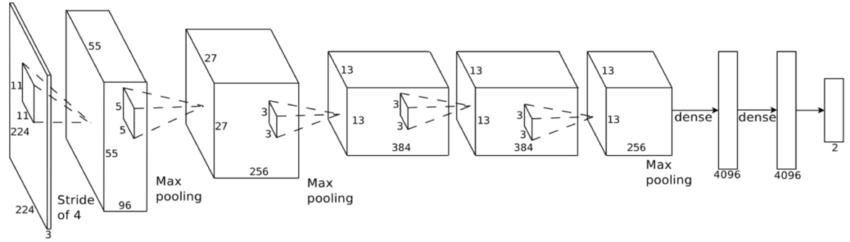
Other than Feed Forward Neural Networks, we also employed the Convolution Neural network model, developed by LeCun et al. [21] to tackle computer vision tasks, CNNs make use of convolution and kernels to perform efficient feature extraction on images. Instead of associating each input pixel with a particular weight, kernels, which are spatially small, are slid (or more formally, convoluted) across the image, extracting features from the image. Additionally, multiple kernels can be used in parallel in a layer, known as the convolution layer, hence allowing each kernel to target different types of features. Then, the features are pooled and downsized, by either taking average or maximum of a patch of features. And this process is repeated several times, generating a tensor, which is then flattened into a vector, then passed onto several feed forward layers. Figure 2 shows AlexNet by Krizhevsky, Sutskever, and Hinton [22], a popular image classifier that makes use of the CNN architecture. However, in our work, we make use of a slightly modified convolution layer, instead of having 2-dimensional kernel and inputs, as in models like AlexNet, we have 1-dimensional kernel and inputs, as the input is a time series data, however the concept is the same.
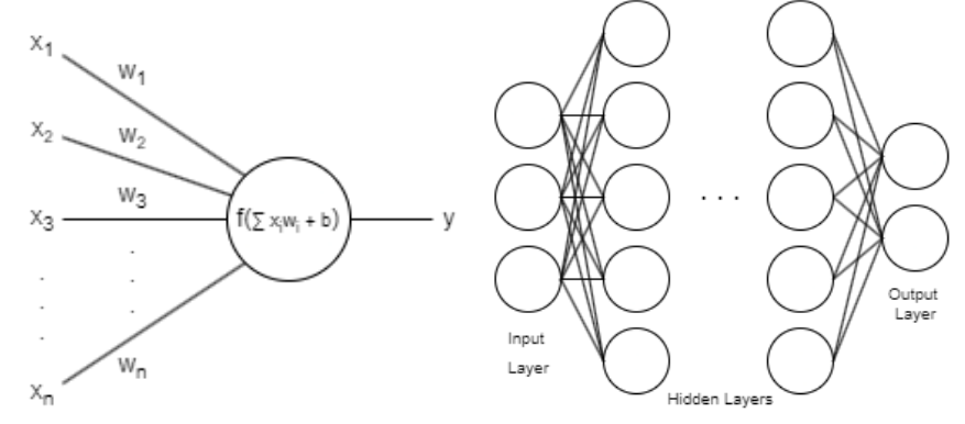
Figure 1. Feed Forward Neural Network model
4. Methodology
We explored multiple machine learning models to tackle the option pricing task that are as follows: we used the classical machine learning model Random Forests, while being simple, they are able to outperform a lot of other both parametric and nonparametric models, we also used the feed forward neural network architecture, a very popular and successful model in various tasks across machine learning, where we modified both the architecture and the training pipeline to improve performance, and we extended our research on neural networks to employ CNNs for better feature extraction, and we also combined multiple models, both parametric and nonparametric, to enhance the accuracy of option pricing.
4.1. Random Forest
Suggested by Ivașcu [8], Random Forest, XGBoost, and LightGMB has all show remarkable performance when compared to other models, and we experimented with combining models, suggested by Das and Padhy [14], but instead of simply learning over outputs of other models, we include the prediction by Black-Scholes, while still having the other inputs, as we hope we can train a “correction” model to yield better results. This idea is further motivated by Shvimer and Zhu [23], where they employed a multi-stage training, the first being pretraining on top of data generated by classical models, so the model can first learn from the classical models, which helps with learning the option prices, while instead of making the model learn from the classical models, we directly provide it as an input for the model as reference, which would eliminate the need to learn from the classical models, and improve the performance. Moreover, as we have a lot of data for our model to train on, the pretraining stage proposed by Shvimer and Zhu [23] is not as necessary. Following Ke and Yang [12], we also predict the ask and bid price separately, which is then averaged out in testing to get the final option price. Overall, the inputs are set to be:
• Underlying stock price
• Strike price
• Maturity
• Risk-free interest rate
• 40-day historical volatility
• Black-Scholes prediction
We implemented our Random Forest Model, which we will use RF to represent, with scikit-learn. With the
4.2. Feed Forward Neural Networks
Similar to Random Forest, we employ similar inputs and outputs for our neural network. And following Ke and Yang [12] and Shvimer and Zhu [23], we also employ feed forward neural networks to tackle the problem. However, we believe that the models tested are not large enough, and with the success of large models in numerous other machine learning tasks such as LLMs in natural language processing, Diffusion models in image generation, CNNs and UNets in computer vision tasks, we decided to use a much deeper and larger model.
Similar to Ke and Yang [12], we used Leaky ReLU as the activation function for all of the layers except for the output layer that predicts the ask and bid price, where we used ReLU instead to ensure the price to be nonnegative. However, in contrast to their work, we did not employ batch normalization, as we did not find it to speed up training, instead, we used a much smaller batch size, 128 instead of 4096.
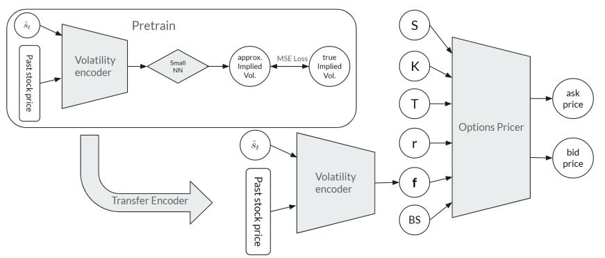
Moreover, we believe that the 40-day historical volatility does not provide enough information about the implied volatility for the model, hence we included both the 20-day and 60-day historical volatility as extra inputs. Furthermore, we also provide the past 40 day stock price in addition to the historical volatilities for the model to possess more information about the stock. And instead of just feeding these information to one large model, as a lot of the input neurons are used to provide the model information of the stock volatility, we employ a smaller volatility encoder module (see Figure 3) to encode all the volatility-related information, which is later concatenated with the other information of the option, and given to the main model, the option pricing module. While it is intuitive to set the volatility encoder to output a single number, that being the implied volatility, we did not see much improvement. We proposed that it can only encode so much information to one neuron, thus we changed it to encode into a volatility feature vector.
With 2 modules and so many parameters, training is significantly harder, especially in the first few epochs when the volatility encoder is not well trained, the features it encoded is very random, which makes learning the option pricer module difficult and ineffective. To combat this, we set up a pre-training stage for the volatility encoder, by hooking it up with a small neural network to predict the implied volatility, which then we transfer the encoder to the option pricer module and train them in parallel (see Figure 3). We find this method to accelerate the training process and reduce the amount of epochs needed to get a satisfactory result.
Additionally, with so many inputs of different ranges, it can be quite hard for the model to learn all the parameters, especially with the same learning rate, hence we also apply a standardization to all inputs beforehand, which we saw huge improvements to the performance. Details of the model, which we will use NN to represent, are summarized in table 1.
|
Layer |
Output Size |
No. of Parameters |
|
Option Pricer |
||
|
Input |
25 |
0 |
|
Hidden 1 |
800 |
20,800 |
|
Hidden 2 |
400 |
320,400 |
|
Hidden 3 |
200 |
80,200 |
|
Hidden 4 |
100 |
20,100 |
|
Output |
2 |
202 |
|
Volatility En-coder |
||
|
Input |
40 |
0 |
|
Hidden 1 |
400 |
16,400 |
|
Hidden 2 |
100 |
20,100 |
|
Hidden 3 |
100 |
10,100 |
|
Output |
20 |
2,020 |
|
Total |
510,322 |
4.3. Convolution Neural Networks
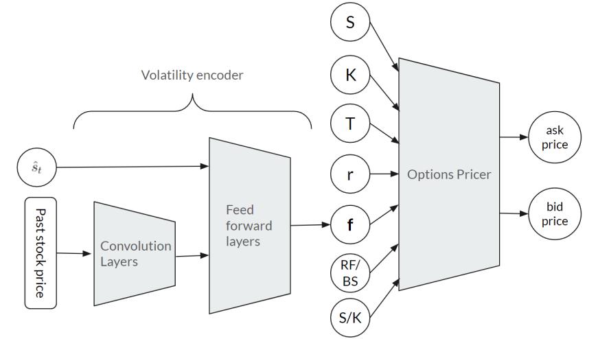
Many work done surrounding option pricing with machine learning have all been focused on feed forward neural networks, Recurrent Neural Networks (RNNs), Long Short Term Memory (LSTM), and other classical machine learning models, no many have explored the possibilities with Convolution Neural Networks (CNNs). Thus we incorporated CNNs into our architecture by adding convolution layers in the volatility encoder module. However instead of just extracting features across the 40-day stock price and the historical volatilities, as the they are features extracted from the past stock prices themselves, we only apply the convolution layers to the 40-day stock price, and flatten the extracted features into a vector, which is them concatenated with the historical volatilities and further process using feed forward layers (see Figure 4). This architecture can allow the kernels from the convolution layers to focus on extracting features from the stock price and do not need to learn about feature extraction from the historical volatilities, which makes them more targeted and thus yielding better performance.
Furthermore, while it is widely popular to use Mean-Squared Error (MSE) as the loss, especially for regression based tasks like this, we notice several downsides of MSE, notably the prioritization of learning to predict outputs that are of larger value in terms of percentage error. As shown in Figure 5A, with the x-axis being the percentage error of the predicted price, and the y-axis being the log of the true price, we see the significant imbalance of the percentage error between the expensive and cheap options.
Hence we designed a regularization term, mean squared percentage error (MSPE), which is computed as (12), and the new loss term is (13), with λ1 being a regularization strength. We have also tried simply using MSPE as the primary loss term instead of the regularization term, but it yielded a model with high MSE and MAE, which we reason to be its prioritization of learning cheaper options in terms of absolute error, and thus the high MSE and MAE. As minimizing absolute error is more important than minimizing percentage error, we decided to include MSPE as a regularization term. Moreover, we set λ1 in (13) to be 0 in the first few epochs, as while the model is still untrained and when the MSE is already large,
We also made other small improvements to the model, notably the addition of another input, moneyness, computed by stock price over strike price, to the option pricer, which we see to be quite helpful and improved the performance significantly. Furthermore, while the last layer uses the ReLU activation function, which ensures the output to be nonnegative, as the gradient can be 0 when the output is 0, which does not allow learning of the model, we modified so that when training, we do not apply the ReLU activation function, and we only apply it during testing. We also included L2-regularization (14), where
|
Layer |
Output Size |
No. of Parameters |
|
Option Pricer |
||
|
Input |
56 |
0 |
|
Hidden 1 |
800 |
45,600 |
|
Hidden 2 |
400 |
320,400 |
|
Hidden 3 |
200 |
80,200 |
|
Hidden 4 |
100 |
20,100 |
|
Output |
2 |
202 |
|
Volatility En-coder |
||
|
Input |
43 |
0 |
|
Conv1+Pool 1 |
205 |
|
|
Conv 2 |
910 |
|
|
Conv3+Pool 2 |
3220 |
|
|
Hidden 1 |
400 |
576,000 |
|
Hidden 2 |
100 |
40,100 |
|
Output |
50 |
5,050 |
|
Total |
573,587 |
5. Data
The data used in this experiment is the SPX 2023 Call options from optionsDX (end of day) [24], which provides us the underlying stock price, strike, maturity, implied volatility, ask and bid prices. And similar to Ke and Yang [12], we used the daily US treasury yield curve provided by the US government [25] as our risk-free interest rate. During preprocessing, we filter out invalid values of each term like options with prices of 0 and negative implied volatility. As a lot of the options are traded in one day, the corresponding maturities are 0, as we only used end of day data, hence these data are also filtered out. After preprocessing, we have nearly 800,000 data points for our model to train, which we split into training dataset, testing dataset, and validation dataset, using a 90% − 5% − 5% split, and we batchify the data using a batch size of 128 with the DataLoader class from PyTorch, using 128 as the seed for easy replication.
6. Performance and analysis
To measure performance and accuracy of a model doing a regression task, 3 metrics are commonly used, mean squared error (MSE), mean absolute error (MAE), and mean absolute percentage error (MAPE), their mathematical formulations are as follows:
We trained NN, CNN-BS, and CNN-RF for 5 epochs in the pre-training stage and in the main training stage, we trained NN for 10 epochs while we trained CNN-BS and CNN-RF for 20 epochs. RF used the default hyperparameters provided by scikit-learn, the learning rate for training NN is 5e-4 for the first 6 epochs, and 1e-4 for the other 4 epochs, and for CNN-BS and CNN-RF, the learning rate is 5e-4 for the first 8 epochs, 1e-4 for epochs 9 to 16, and 2e-5 for the last 4 epochs, with λ1 set to 0 for the first 8 epochs and 5e-2 for the rest, and λ2 is set to 5e-5 for all 20 epochs. Table 3 shows a comparison of the performance of each model using the 3 metrics, with the best performing model bolded, with Black-Scholes as the baseline.
|
Model |
RMSE |
MAE |
MAPE |
|
Black-Scholes |
68.3 |
42.0 |
31.6% |
|
RF |
4.2 |
2.5 |
2.1% |
|
NN |
4.3 |
1.8 |
2.7% |
|
CNN-RF |
3.2 |
1.9 |
1.8% |
|
CNN-3S |
2.2 |
1.2 |
1.9% |
We see that CNN-BS and CNN-RF outperforms all other models tested, and RF, despite its simplicity, performs significantly better than NN, which is in line with Ivașcu [8]. Additionally, it is rather surprising that CNN-BS outperforms CNN-RF in terms of RMSE and MAE as Random Forest performs significantly better than Black-Scholes, and hence we expected that it would be a much more accurate reference of the true price for the CNN model. However, further analysis in the model performance shows that CNN-RF indeed performs much better than CNN-BS, but only in terms of the training dataset, thus we believe that CNN-RF performs worse than CNN-BS as a result of Random Forest, despite being much more accurate than Black-Scholes, is more prone to overfitting, and that more measure to prevent overfitting needs to be implemented.
However, we still demonstrated the effectiveness of the extra regularization terms based on the model CNN-RF, even with hyperparameters that are not fine tuned, through Table 4. We can still see some improvements in RMSE, MAE, and MAPE, hence showing that our regularization terms have some level of effectiveness. And in Figure 5B, we plotted the percentage error of the predicted price to the log (base 10) of the true price for the CNN-RF with and without the MSPE regularization. We can see that for cheap options, the percentage errors are much smaller, and we believe with better fine-tuned regularization strength, the effect can be significantly amplified.
Despite our regularization attempts, more work has to be done, in both the bal-ancing of percentage errors across different price ranges and the overfitting issue in large models. Other than the overfitting issue in CNN-RF, we also saw some similar problems in both NN and CNN-BS, while the loss of the testing dataset is similar to that of the training dataset, which is in line with Ke and Yang [12], we notice the significant discrepancy of the training loss and validation loss, as presented in Figures 6A and 6B.
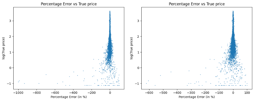
Figure 5. Percentage error of the predicted price to the log (base 10) of the true price for CNN-RF with and without MSPE regularization
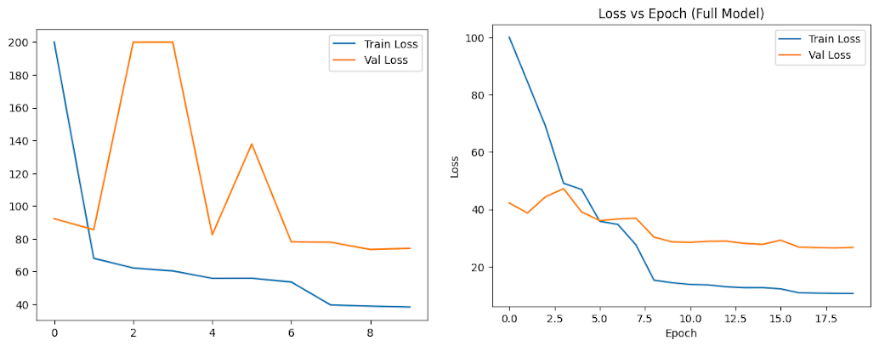
B. Loss of the training dataset and validation dataset for CNN-RF
Figure 6. Comparision between the loss of the training dataset and validation dataset (Capped at 200)
|
Model |
RMSE |
MAE |
MAPE |
|
CNN-RF |
3.20 |
1.87 |
1.81% |
|
3.26 |
1.92 |
1.97% |
|
|
3.25 |
1.91 |
1.83% |
Furthermore, we also trained all of the models on different seeds, and yet such discrepancy still existed. While the L2-regularization term can partially solve the issue, there is still a lot of work to be done with other preventative measures of overfitting such as dropout.
7. Conclusion
In conclusion, we have presented several nonparametric models in this paper, with all models have significantly outperformed the Black-Scholes model, we showcased the potential of classical machine learning, deep learning, and combinations of both with parametric modeling in the task of option pricing. Future work can consider combining multiple models, both parametric and nonparametric, and can incorporate other solutions of overfitting for large models like those presented in this paper. Regarding neural network architectural types, we have presented lesser explored models such as CNNs and showcased the potential compared to traditional neural networks and RNNs/LSTMs.
However, due to the time limit, we are not able to fully demonstrate the potential of our regularization efforts, which could be done with better fine tuning, and with more time, we wish to explore other model architectures, we can also conduct more analysis such as bias of our model predictions and the effectiveness of each aspect of our models, and we can also extend our model architecture to put options, other option types, and to data ranging longer timespans, we can even experiment with more generalized models that can handle multiple stocks, instead of being tailored to one.
Acknowledgement
Peter Hong Zhi Liu and Jiaxi Dai contributed equally to this work and should be considered co-first authors.
References
[1]. Black, F., & Scholes, M. (1973). The pricing of options and corporate liabilities. Journal of political economy, 81(3), 637-654.
[2]. Heston, S. L. (1993). A closed-form solution for options with stochastic volatility with applications to bond and currency options. The review of financial studies, 6(2), 327-343.
[3]. Merton, R. C. (1976). Option pricing when underlying stock returns are discontinuous. Journal of financial economics, 3(1-2), 125-144.
[4]. Dupire, B. (1994). Pricing with a smile. Risk, 7(1), 18-20.
[5]. Bates, D. S. (1996). Jumps and stochastic volatility: Exchange rate processes implicit in deutsche mark options. The Review of Financial Studies, 9(1), 69-107.
[6]. Bakshi, G., Cao, C., & Chen, Z. (1997). Empirical performance of alternative option pricing models. The Journal of finance, 52(5), 2003-2049.
[7]. Hutchinson, J. M., Lo, A. W., & Poggio, T. (1994). A nonparametric approach to pricing and hedging derivative securities via learning networks. The journal of Finance, 49(3), 851-889.
[8]. Ivașcu, C. F. (2021). Option pricing using machine learning. Expert Systems with Applications, 163, 113799.
[9]. Amilon, H. (2003). A neural network versus Black-Scholes: a comparison of pricing and hedging performances. Journal of Forecasting, 22(4), 317–335.
[10]. Yang, S. H., & Lee, J. (2011). Predicting a distribution of implied volatilities for option pricing. Expert Systems with Applications, 38(3), 1702-1708.
[11]. Liu, S., Oosterlee, C. W., & Bohte, S. M. (2019). Pricing options and computing implied volatilities using neural networks. Risks, 7(1), 16.
[12]. Ke, A., & Yang, A. (2019). Option pricing with deep learning. Department of Computer Science, Standford University, In CS230: Deep learning, 8, 1-8.
[13]. Glau, K., & Wunderlich, L. (2022). The deep parametric PDE method and applications to option pricing. Applied Mathematics and Computation, 432, 127355.
[14]. Das, S. P., & Padhy, S. (2017). A new hybrid parametric and machine learning model with homogeneity hint for European-style index option pricing. Neural Computing and Applications, 28, 4061-4077.
[15]. Breiman, L. (2001). Random forests. Machine learning, 45, 5-32.
[16]. Breiman, L., Friedman, J., Olshen, R., & Stone, C. (1984). Cart. Classification and regression trees.
[17]. Breiman, L. (1996). Bagging predictors. Machine learning, 24, 123-140.
[18]. McCulloch, W. S., & Pitts, W. (1943). A logical calculus of the ideas immanent in nervous activity. The bulletin of mathematical biophysics, 5, 115-133.
[19]. Nair, V., & Hinton, G. E. (2010). Rectified linear units improve restricted boltzmann machines. In Proceedings of the 27th international conference on machine learning (ICML-10) (pp. 807-814).
[20]. Maas, A. L., Hannun, A. Y., & Ng, A. Y. (2013, June). Rectifier nonlinearities improve neural network acoustic models. In Proc. icml (Vol. 30, No. 1, p. 3)
[21]. LeCun, Y., Bottou, L., Bengio, Y., & Haffner, P. (1998). Gradient-based learning applied to document recognition. Proceedings of the IEEE, 86(11), 2278-2324.
[22]. Krizhevsky, A., Sutskever, I., & Hinton, G. E. (2012). Imagenet classification with deep convolutional neural networks. Advances in neural information processing systems, 25.
[23]. Shvimer, Y., & Zhu, S. P. (2024). Pricing options with a new hybrid neural network model. Expert Systems with Applications, 251, 123979.
[24]. OptionsDX. (2023). OptionsDX 2023 SPX EOD Data. https: //www.optionsdx.com/product/spx-option-chain/., Accessed: 2024-06-10.
[25]. U. S. Department of the Treasury. (2023). U.S. Treasury Daily Par Yield Curve. https: //home.treasury.gov/resource-center/data-chart-center/interest-rates/TextView?type=daily_treasury_yield_curve& field_tdr_date_value=2023, Accessed: 2024-06-10
Cite this article
Liu,P.H.Z.;Dai,J. (2025). Options Pricing with Various Machine Learning Models. Advances in Economics, Management and Political Sciences,202,225-237.
Data availability
The datasets used and/or analyzed during the current study will be available from the authors upon reasonable request.
Disclaimer/Publisher's Note
The statements, opinions and data contained in all publications are solely those of the individual author(s) and contributor(s) and not of EWA Publishing and/or the editor(s). EWA Publishing and/or the editor(s) disclaim responsibility for any injury to people or property resulting from any ideas, methods, instructions or products referred to in the content.
About volume
Volume title: Proceedings of the 3rd International Conference on Financial Technology and Business Analysis
© 2024 by the author(s). Licensee EWA Publishing, Oxford, UK. This article is an open access article distributed under the terms and
conditions of the Creative Commons Attribution (CC BY) license. Authors who
publish this series agree to the following terms:
1. Authors retain copyright and grant the series right of first publication with the work simultaneously licensed under a Creative Commons
Attribution License that allows others to share the work with an acknowledgment of the work's authorship and initial publication in this
series.
2. Authors are able to enter into separate, additional contractual arrangements for the non-exclusive distribution of the series's published
version of the work (e.g., post it to an institutional repository or publish it in a book), with an acknowledgment of its initial
publication in this series.
3. Authors are permitted and encouraged to post their work online (e.g., in institutional repositories or on their website) prior to and
during the submission process, as it can lead to productive exchanges, as well as earlier and greater citation of published work (See
Open access policy for details).
References
[1]. Black, F., & Scholes, M. (1973). The pricing of options and corporate liabilities. Journal of political economy, 81(3), 637-654.
[2]. Heston, S. L. (1993). A closed-form solution for options with stochastic volatility with applications to bond and currency options. The review of financial studies, 6(2), 327-343.
[3]. Merton, R. C. (1976). Option pricing when underlying stock returns are discontinuous. Journal of financial economics, 3(1-2), 125-144.
[4]. Dupire, B. (1994). Pricing with a smile. Risk, 7(1), 18-20.
[5]. Bates, D. S. (1996). Jumps and stochastic volatility: Exchange rate processes implicit in deutsche mark options. The Review of Financial Studies, 9(1), 69-107.
[6]. Bakshi, G., Cao, C., & Chen, Z. (1997). Empirical performance of alternative option pricing models. The Journal of finance, 52(5), 2003-2049.
[7]. Hutchinson, J. M., Lo, A. W., & Poggio, T. (1994). A nonparametric approach to pricing and hedging derivative securities via learning networks. The journal of Finance, 49(3), 851-889.
[8]. Ivașcu, C. F. (2021). Option pricing using machine learning. Expert Systems with Applications, 163, 113799.
[9]. Amilon, H. (2003). A neural network versus Black-Scholes: a comparison of pricing and hedging performances. Journal of Forecasting, 22(4), 317–335.
[10]. Yang, S. H., & Lee, J. (2011). Predicting a distribution of implied volatilities for option pricing. Expert Systems with Applications, 38(3), 1702-1708.
[11]. Liu, S., Oosterlee, C. W., & Bohte, S. M. (2019). Pricing options and computing implied volatilities using neural networks. Risks, 7(1), 16.
[12]. Ke, A., & Yang, A. (2019). Option pricing with deep learning. Department of Computer Science, Standford University, In CS230: Deep learning, 8, 1-8.
[13]. Glau, K., & Wunderlich, L. (2022). The deep parametric PDE method and applications to option pricing. Applied Mathematics and Computation, 432, 127355.
[14]. Das, S. P., & Padhy, S. (2017). A new hybrid parametric and machine learning model with homogeneity hint for European-style index option pricing. Neural Computing and Applications, 28, 4061-4077.
[15]. Breiman, L. (2001). Random forests. Machine learning, 45, 5-32.
[16]. Breiman, L., Friedman, J., Olshen, R., & Stone, C. (1984). Cart. Classification and regression trees.
[17]. Breiman, L. (1996). Bagging predictors. Machine learning, 24, 123-140.
[18]. McCulloch, W. S., & Pitts, W. (1943). A logical calculus of the ideas immanent in nervous activity. The bulletin of mathematical biophysics, 5, 115-133.
[19]. Nair, V., & Hinton, G. E. (2010). Rectified linear units improve restricted boltzmann machines. In Proceedings of the 27th international conference on machine learning (ICML-10) (pp. 807-814).
[20]. Maas, A. L., Hannun, A. Y., & Ng, A. Y. (2013, June). Rectifier nonlinearities improve neural network acoustic models. In Proc. icml (Vol. 30, No. 1, p. 3)
[21]. LeCun, Y., Bottou, L., Bengio, Y., & Haffner, P. (1998). Gradient-based learning applied to document recognition. Proceedings of the IEEE, 86(11), 2278-2324.
[22]. Krizhevsky, A., Sutskever, I., & Hinton, G. E. (2012). Imagenet classification with deep convolutional neural networks. Advances in neural information processing systems, 25.
[23]. Shvimer, Y., & Zhu, S. P. (2024). Pricing options with a new hybrid neural network model. Expert Systems with Applications, 251, 123979.
[24]. OptionsDX. (2023). OptionsDX 2023 SPX EOD Data. https: //www.optionsdx.com/product/spx-option-chain/., Accessed: 2024-06-10.
[25]. U. S. Department of the Treasury. (2023). U.S. Treasury Daily Par Yield Curve. https: //home.treasury.gov/resource-center/data-chart-center/interest-rates/TextView?type=daily_treasury_yield_curve& field_tdr_date_value=2023, Accessed: 2024-06-10