1. Introduction

In modern society, with the development of quantitative investment, how to achieve effective risk control when pursuing returns has become a core issue in asset allocation strategies. Within many quantitative strategies, momentum strategies are widely used because of their strong predictive ability. These strategies typically rely on historical returns to identify assets with recent strong performance. However, most traditional momentum strategies rely on the Sharpe Ratio to measure performance. This indicator is based on total volatility and fails to effectively distinguish between upside and downside risks, especially in extreme market situations such as COVID-19, there is a significant lack of control over tail risks. In recent years, the academic community has proposed the stable tail adjusted return ratio (STARR) based on conditional value at risk (CVaR) as a more stable risk-adjusted return indicator. Unlike the Sharpe Ratio, STARR measures the expected return corresponding to each unit of extreme downside risk (as measured by CVaR), which can better reflect the stability of the strategy when the market fluctuates violently. Rachev et al. demonstrated that momentum strategies built on reward–risk ratios such as STARR provide stronger downside protection under extreme market environments and outperform cumulative return-based strategies [1]. Although STARR has obvious advantages in risk control, most of the current related research is limited to the individual stock level, and less attention is paid to the heterogeneity between different industries. However, there are significant differences in volatility, systemic risk exposure, policy sensitivity, etc. between different industries, which may affect the effectiveness of momentum signals and tail risk control. Therefore, this paper uses Nikkei 225 and S&P 500 as industry ETF data representing the Japanese and US markets to systematically evaluate the performance differences of the STARR momentum strategy in different industries and markets and introduces the mean-variance optimization method to control the overall volatility of the portfolio and further improve the stability of the strategy. This research aims to evaluate the STARR-based momentum strategy's effectiveness across heterogeneous industries under uncertain market conditions.

2. Literature review

Li et al. provided evidence and explanations for the momentum effect in the world, highlighting its significance across various cultural and economic contexts [2]. A considerable amount of research suggests that disproportionate gains can be harvested using momentum investment strategies over various regions and epochs, thus resulting in one of the significant factor models of quantitative investment. Hofmann and Keiber explored seasonality effects in the German stock market, suggesting that momentum strategies may exhibit time-dependent patterns [3]. The STARR indicator based on CVaR can be used to measure the expected return corresponding to tail risk and is therefore widely used in portfolio management in extreme situations. At the level of industry, Moskowitz and Grinblatt emphasized the predictability benefits associated with industry-level momentum signals [4]. Individually, the bulk of stock momentum returns stem from the momentum effect at the industry level. When the industry component is removed, the individual stock momentum returns considerably diminished or vanishes altogether. On the other hand, the industry-level momentum strategy is more resilient and explanative, as it continues to yield considerable excess returns even after multiple risk factors are considered. Industry characteristics such as volatility, policy sensitivity and economic cycle response will have a significant impact on the performance and risk characteristics of factors. Additionally, Gao et al. examined how investor heterogeneity influences momentum-based strategies, especially in emerging markets, revealing that risk preferences and market participation vary significantly across industries [5]. Lin further confirmed the existence of robust industry-level momentum in the A-share market, emphasizing the role of industry rotation in generating excess returns [6].

3. Data preparation

This research constructs industry-level datasets for the U.S. and Japanese markets, respectively, based on monthly closing prices from January 2010 to June 2025. For the US market, 20 GICS secondary industry ETFs (such as Energy–XLE, Materials–XLB, Utilities–XLU, Semiconductors–SMH, etc.) were selected. For the Japanese market, 17 NEXT FUNDS industry ETFs (such as 1618.T Energy, 1629.T Commerce, 1627.T Utilities, etc.) were selected. The monthly closing prices of all notes were downloaded in batches through yahoo finance by getting the data of the last trading day of each month and aligned them by date.

First, for the monthly data of constituent stocks obtained, all sector ETFs with more than 20% missing observations in the sample are excluded—a criterion that results in the removal of three US sector ETFs, leaving 17 US sector series and 17 Japanese sector series. Second, for the remaining assets, isolated gaps of up to two consecutive months are filled using linear interpolation; series with longer gaps are removed entirely. Third, to mitigate the impact of extreme price spikes or plunges, each price series is converted to a z-score, and any observation that any observation with an absolute z-score greater than 3 was excluded.

The cleaned closing price data of each ETF (and the two benchmark indices) are then reassembled into a T×N matrix, where T is the number of month-end dates and N=36 is the total number of retained sequences. This matrix has no major gaps and extreme distortions, providing a solid foundation for calculating log returns, constructing momentum factors (Sharp and STARR), and subsequent portfolio optimization and performance analysis.

4. Strategy design

4.1. Method

This section is based on the monthly closing prices of industry ETFs, using Sharpe and STARR momentum factors as trading signals, and uses the mean-variance (M-V) optimization model to strengthen risk control and complete strategy construction, evaluation, and parameter optimization.

4.1.1. Return and factor calculation

First, convert the month-end closing price of each industry ETF into logarithmic returns by Log Return Formula. the research constructs two types of momentum factors at the end of each month based on the return series of the past T=6 months to capture the relative strength and tail risk characteristics of industries. Specifically, the annualized average return of the i-th ETF at the end of the month at time t is defined as

$$ {\mathrm{r}}_{\mathrm{i},\mathrm{t}}=\mathrm{l}\mathrm{n}\frac{{\mathrm{P}}_{\mathrm{i},\mathrm{t}}}{{\mathrm{P}}_{\mathrm{i},\mathrm{t}-1}}$$(1)

In this formula, where  $$ {\mathrm{P}}_{\mathrm{i},\mathrm{t}}\mathrm{ }\mathrm{a}\mathrm{n}\mathrm{d}\mathrm{ }{\mathrm{P}}_{\mathrm{i},\mathrm{t}-1}$$  are the closing prices at the end of month t and t-1 respectively. Unlike simple yields, logarithmic yields are time-additive, meaning they can be aggregated over multiple periods can be directly added together, which greatly facilitates statistics and modeling within the rolling window. In addition, after taking the logarithm, it is less sensitive to extreme values ​​and is closer to the normal distribution assumption, thus improving the robustness of many financial models in parameter estimation and risk measurement.

Based on this sequence,the research calculates the annualized average return.

$$ {\stackrel{-}{\mathrm{R}}}_{\mathrm{i},\mathrm{t}}=\frac{12}{\mathrm{T}}\sum _{\mathrm{k}=0}^{\mathrm{T}-1}{\mathrm{r}}_{\mathrm{i},\mathrm{t}-\mathrm{k}}$$(2)

And the annualized volatility,

$$ {\mathrm{\sigma }}_{\mathrm{i}}=\stackrel{-}{\frac{12}{\mathrm{T}-1}\left({\sum _{\mathrm{k}=0}^{\mathrm{T}-1}\left({\mathrm{r}}_{\mathrm{i},\mathrm{t}-\mathrm{k}}-\frac{\stackrel{-}{{\mathrm{R}}_{\mathrm{i}}}}{12}\right)}^2\right)}$$(3)

4.1.2. Momentum factor construction

Based on these statistics, the research first define the common Sharpe-based momentum factor:

$$ {\mathrm{S}\mathrm{h}\mathrm{a}\mathrm{r}\mathrm{p}\mathrm{e}}_{\mathrm{i},\mathrm{t}}=\frac{{\stackrel{-}{\mathrm{R}}}_{\mathrm{i},\mathrm{t}}}{{\mathrm{\sigma }}_{\mathrm{i},\mathrm{t}}}$$(4)

To measure the excess return capability under unit overall volatility. However, since pure volatility cannot reflect extreme downside risk.

At the same time, the research estimate the average loss ( $$ {\mathrm{C}\mathrm{V}\mathrm{a}\mathrm{R}}_{95\mathrm{\%}}$$ )

$$ \mathrm{S}\mathrm{T}\mathrm{A}\mathrm{R}{\mathrm{R}}_{\mathrm{i}}=\frac{{\stackrel{-}{\mathrm{R}}}_{\mathrm{i}}}{{\mathrm{C}\mathrm{V}\mathrm{a}\mathrm{R}}_{95\mathrm{\%}}}$$(5)

 $$ {\mathrm{C}\mathrm{V}\mathrm{a}\mathrm{R}}_{95\mathrm{\%}}$$  represents the average loss under the worst 5% of returns in the first 6 months. Its estimation process first sorts the return sequence in ascending order, then takes the arithmetic average of the first 0.05T negative values and truncates the value to prevent numerical instability due to an excessively small denominator.

To test the sensitivity of the factors to parameter settings, in addition to the benchmark 6-month formation period, the research also tested 3-month and 12-month sliding windows in the empirical test. The results show that the 6-month window is the best in balancing signal response speed and volatility smoothing, while the short window is susceptible to occasional extreme shocks, and the long window is slow to respond to emerging momentum opportunities. The above multiple factor construction and parameter testing provide a solid statistical basis for the selection and weight optimization of the strategy. CVaR satisfies the four coherence axioms introduced by Artzner et al., making it a robust choice for tail risk estimation in financial modeling [7].

4.1.3. Factor standardization and sorting

To ensure the comparability of different factors across different industries, the research perform Z-Score normalization on the Sharpe and STARR factor values ​​that are not obtained each month:

$$ {\tilde{\mathrm{F}}}_{\mathrm{i},\mathrm{t}}=\frac{{\mathrm{F}}_{\mathrm{i},\mathrm{t}}-{\mathrm{\mu }}_{\mathrm{F},\mathrm{t}}}{{\mathrm{\sigma }}_{\mathrm{F},\mathrm{t}}}$$(6)

Among them,  $$ {\mathrm{F}}_{\mathrm{i},\mathrm{t}}$$  represents the original factor value and  $$ {\mathrm{\mu }}_{\mathrm{F},\mathrm{t}}$$  and  $$ {\mathrm{\sigma }}_{\mathrm{F},\mathrm{t}}$$  are the cross-industry mean and standard deviation of the current factor, respectively. After standardization, the 20 industry ETFs are sorted from high to low according to  $$ {\tilde{\mathrm{F}}}_{\mathrm{i},\mathrm{t}}$$ , and the top 5 scores are selected to form the current "winner pool".

4.1.4. Portfolio construction and mean-variance optimization

After completing the factor sorting and selecting the top five industry ETFs with the highest scores, the research designed two different fund allocation plans. The first plan is equal-weight allocation, which means allocating available capital equally to each selected ETF. It is simple, intuitive and easy to implement. The second plan introduces the idea of ​​risk optimization: the research uses the mean return and covariance information of these five ETFs in the past six months, combined with investors' tolerance for overall volatility and the upper limit requirements for the weight of a single industry, to calculate a set of optimal weights to maximize the expected return of the portfolio while meeting the established risk constraints. This process also considers the transaction costs brought about by each rebalancing (assuming 0.1% in both directions) to ensure that the optimization results are feasible in both theory and practice. Finally, both plans will be rebalanced at the end-of-month closing price on the first trading day of each month and will be maintained until the next rebalancing day for subsequent backtesting and performance comparison. Imran et al. analyzed momentum effects in developed and emerging stock markets, offering cross-country insights that complement industry-level analyses [8].

4.2. Evaluation method

4.2.1. Performance indicators

After the backtest, the research construct a net asset value sequence based on the monthly portfolio yield:

$$ {\mathrm{V}}_{\mathrm{t}}={\mathrm{V}}_{\mathrm{t}-1}\left(1+{\mathrm{r}}_{\mathrm{p},\mathrm{t}}\right),\mathrm{ }{\mathrm{V}}_0=1$$(7)

And calculate the two core indicators of annualized yield and Sharpe ratio. The annualized yield is in the form of geometric compounding:

$$ {\mathrm{R}}_{\mathrm{a}\mathrm{n}\mathrm{n}}={\left(\prod _{\mathrm{t}=1}^{\mathrm{T}}\left(1+{\mathrm{r}}_{\mathrm{p},\mathrm{t}}\right)\right)}^{\frac{12}{\mathrm{T}}}-1$$(8)

Where  $$ \mathrm{T}$$  is the total number of backtest months; the Sharpe ratio is measured by the ratio of average excess return internalized to annualized volatility, reflecting the profitability under unit risk. On this basis, the research also report the maximum drawdown to examine the maximum loss under extreme market conditions, and the STARR ratio to characterize the return performance corresponding to each unit of tail risk. The above indicators can concisely and comprehensively reflect the risk-return characteristics of the strategy. Following Guo and Ryan, the use of CVaR and STARR improves risk control, especially during momentum crash-prone periods [9].

4.2.2. Robustness test

To verify the robustness of the strategy under different market environments and parameter configurations,the research designed multi-dimensional sub-samples and scenario analysis. First, the full sample was divided into two stages: pre-epidemic (2010–2019) and post-epidemic (2020–2025), and the annualized return, volatility, Sharpe and STARR ratios, and maximum drawdown of each period were calculated to examine the impact of extreme shocks on the performance of the strategy. Second, according to the median market volatility, the high volatility period and the low volatility period were divided, and the risk-adjusted returns under the two environments were compared. Third, sensitivity tests were conducted in the two dimensions of formation period (3, 6, and 12 months) and holding period (1 and 3 months). Through grid search, the Sharpe, STARR, MDD (Maximum Drawdown), and IR (Information Ratio) indicators of each parameter combination were recorded respectively to evaluate the stability of the strategy to parameter changes. Through the above multiple tests, it is ensured that the industry momentum strategy designed based on Sharpe and STARR factors can maintain robust risk-return characteristics in different markets, different stages, and different settings.

4.3. Parameter optimization and cross-market verification

In the parameter optimization phase, the research conducted a grid search on four dimensions: formation period, holding period, number of selected stocks (top 5, 8, 10), and annualized volatility cap (8%, 10%, 12%). First, the research screened out a batch of parameters with the best performance and the smallest volatility in indicators such as Sharpe, STARR, and maximum drawdown from the internal sample of 2010.1–2021.12; then the research verified its robustness in the external sample of 2022.1–2025.4. Finally, the optimal parameters that passed the dual test of internal and external samples were applied to the S&P 500 and Nikkei 225 industry ETF data to evaluate the versatility and consistency of the strategy in different market environments.

5. Study performance

5.1. Comparison of strategy effectiveness in different markets

Table 1 reports the key performance metrics of the four momentum strategies applied to the S&P 500 and Nikkei 225 industry ETFs over the period 2010.01 to 2025.04. In the US market, the Sharpe Equal Weight strategy achieved the highest annualized return (11.94%), but also the highest annualized volatility (14.29%) and maximum drawdown (–16.93%). After introducing Mean-Variance optimization, Sharpe Mean-Variance slightly reduced the volatility to 14.14%, but the return and drawdown were under pressure. The STARR factor also performed well under equal weight allocation with annualized return 11.38%, volatility 14.14%, maximum drawdown –16.22%, while STARR Mean-Variance was slightly better than Sharpe Mean-Variance in controlling drawdown (–17.37% vs. –19.28%) and maintained a higher risk-adjusted return with Sharpe ratio of 71.76%. Zaremba confirmed the presence of momentum effects at the country level across global stock markets [10].

In the Japanese market, the annualized returns of the four strategies are relatively low, among which STARR Equal Weight reaches 9.02%, with a volatility of 14.07% and a maximum drawdown of -26.09%. After Mean-Variance optimization, STARR Mean-Variance reduces the maximum drawdown to -24.24%, and the annualized volatility drops to 13.61%. In general, Mean-Variance optimization can significantly reduce tail risk in both markets, and the STARR factor is particularly effective in downside protection in the Japanese market.

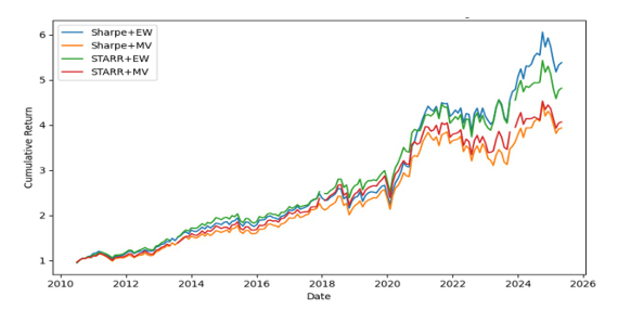
In the S&P 500 market (figure 1), Sharpe+EW achieved a cumulative growth of about 6 times with the highest annualized rate of return; STARR+EW was second, reaching about 5.4 times; although the MV optimization strategy had a lower terminal value (Sharpe+MV ≈ 4.9 times, STARR+MV ≈ 4.1 times), the curve was smoother, and the retracement was smaller.

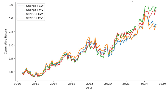
In the Nikkei 225 market (figure 2), STARR+EW has the highest final value, about 3.45 times; STARR+MV, Sharpe+MV and Sharpe+EW are 3.22, 3.10 and 2.80 times respectively. MV optimization also significantly reduces the drawdown and improves the stability of the equity curve.

5.2. Performance before and after the pandemic

To examine the performance differences of the STARR + MV strategy before and after major systemic events, this study uses January 2020 as the dividing point, divides the sample into two stages: pre-epidemic (2010–2019) and post-epidemic (2020–2025.4), and calculates the annualized return, annualized volatility, and rolling 6-month maximum drawdown of the two periods (see Table 2).

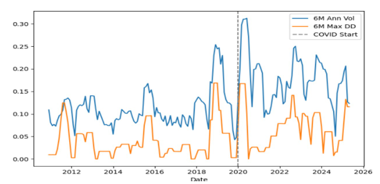
In the US market, the STARR + MV strategy achieved an annualized return of 11.05%, an annualized volatility of 11.59%, and a rolling maximum drawdown of 16.88% before the epidemic; after the epidemic, the annualized return dropped sharply to 6.74%, the volatility increased markedly to 17.96%, and the maximum drawdown also slightly expanded to 17.37%. The rolling 6-month volatility line in Figure 3 rose sharply in early 2020 and remained high all the way. Together with the drawdown curve, it shows that the downward pressure on the strategy under the impact of the epidemic has significantly increased.

In contrast, the performance of the STARR + MV strategy in the Japanese market has rebounded after the epidemic. The annualized return before the epidemic was only 6.99%, the volatility was 14.06%, and the maximum retracement was 24.24%; after the epidemic, the annualized return increased to 11.84%, the volatility fell to 12.83%, and the maximum retracement was significantly narrowed to 7.46%.

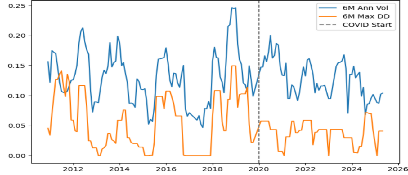
As can be seen in Figure 4, the favorable factors in the Japanese market pushed the strategy to recover rapidly after 2020, and both volatility and retracement were far lower than the pre-epidemic levels.

This result shows that the COVID-19 impact on the U.S. market caused a sharp short-term decline and continued high volatility, which put significant pressure on the strategy's performance. However, the Japanese market experienced a stronger rebound and sustained bull market after the epidemic, allowing the STARR + MV strategy to recover and exceed the pre-epidemic risk-return level in a relatively short period of time.

5.3. Performance in high/low volatility environments

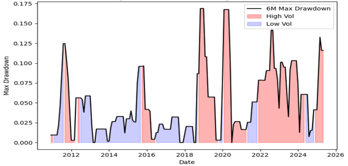
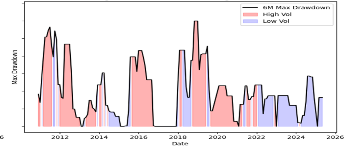
Based on the above, the research uses the median of the rolling six-month annualized volatility of the equal-weighted index at the end of the previous month as the threshold, divide the sample period into high volatility period and low volatility period, and compare the performance of the STARR+MV strategy in the two major markets (see Table 3 and 4).

In the S&P 500 market, the annualized return in the high volatility period reached 12.04%, the annualized volatility was 15.93%, and the maximum six-month drawdown was 17.56%; in the low volatility period, the annualized return fell back to 8.16%, the volatility dropped to 11.96%, but the maximum drawdown slightly increased to 18.09%. In the Nikkei 225 market, the annualized return during the high volatility period was 9.34%, the annualized volatility was 13.72%, and the maximum drawdown was 14.11%; the annualized return during the low volatility period narrowed to 8.00%, the annualized volatility slightly dropped to 13.57%, and the maximum drawdown further narrowed to 12.93%.

As shown in Figures 5 and 6, drawdowns during high-volatility periods (shaded in red) are visibly deeper than those during low-volatility periods (blue), highlighting the STARR+MV strategy’s strong downside protection across different market regimes.

6. Summary

6.1. Model advantages

The STARR+MV framework brings several improvements over traditional return-oriented momentum strategies. First, by embedding a linearized CVaR-based tail‐risk adjustment directly into the factor, it delivers explicit protection against extreme losses without relying on symmetric return assumptions or encountering numerical instabilities when the risk denominator approaches zero. Second, coupling this tail‐aware signal with a mean–variance optimizer allows the model to cap portfolio volatility while simultaneously suppressing deep drawdowns, as demonstrated during the COVID-19 crash in both the S&P 500 and Nikkei 225. Third, because the STARR ratio is linearized, factor values remain smoothly behaved and optimization converges reliably, even in stressed market conditions. Finally, the use of industry ETFs leverages sectoral diversification and enhances practical implement ability, making the strategy both robust and scalable across major equity markets.

6.2. Model disadvantages and future improvements

Despite the significant advantages of the model, the current implementation still has some limitations. The emphasis on tail risk aversion sometimes penalizes high-momentum assets, thereby reducing their upside potential. An effective remedy is to combine the STARR signal with complementary quality indicators (such as profitability or valuation ratios) so that strong fundamentals can mitigate excessive downside penalties. In addition, the static choice of CVaR confidence level and risk aversion coefficient may not be suitable for all market regimes. Introducing dynamic adjustment mechanisms, such as linking risk penalties to realized volatility or macro-regime indicators, can enable the model to reduce the level of protection when the market is calm and increase it when the market is turbulent. Finally, the research’s backtest assumes frictionless trading: incorporating realistic transaction costs, liquidity constraints, and turnover restrictions is critical to estimating net performance and ensuring that the strategy remains implementable under realistic market frictions and liquidity constraints.

References

[1]. Rachev, S.T., Jasić, T., Stoyanov, S.V., and Fabozzi, F.J. (2007). Momentum strategies based on reward–risk stock selection criteria. Journal of Banking & Finance, 31(8), 2325–2346.
[2]. Li, Y., Wang, X., & Zeng, Z. (2021, December). Evidences and explanations for the momentum effect in the world: A literature review. In 2021 3rd International Conference on Economic Management and Cultural Industry (ICEMCI 2021) (pp. 1697-1703). Atlantis Press.
[3]. Hofmann, D., & Keiber, K. L. (2021). Seasonalities in the German stock market. Financial Markets and Portfolio Management, 35(2), 151-192.
[4]. Moskowitz, T. J., & Grinblatt, M. (1999). Do industries explain momentum? The Journal of finance, 54(4), 1249-1290.
[5]. Gao, Y., Han, X., Li, Y., & Xiong, X. (2021). Investor heterogeneity and momentum-based trading strategies in China. International Review of Financial Analysis, 74, 101654.
[6]. Lin, G. (2022, December). Industry Momentum Strategies in A-shares Market. In 2022 International Conference on Economics, Smart Finance and Contemporary Trade (ESFCT 2022) (pp. 1123-1130). Atlantis Press.
[7]. Artzner, P., Delbaen, F., Eber, J. M., & Heath, D. (1999). Coherent measures of risk. Mathematical finance, 9(3), 203-228.
[8]. Imran, Z. A., Wong, W. C., & Ismail, R. (2020). Momentum Effect in Developed and Emerging Stock Markets. Journal of Finance and Accounting Research, 2(2), 14-31.
[9]. Guo, X., & Ryan, S. M. (2023). Avoiding momentum crashes using stochastic mean-CVaR optimization with time-varying risk aversion. The Engineering Economist, 68(3), 125-152.
[10]. Zaremba, A. (2018). The momentum effect in country-level stock market anomalies. Economic research-Ekonomska istraživanja, 31(1), 703-721.
Cite this article
Zhang,X. (2025). Risk-adjusted Momentum Strategy Construction and Industry Heterogeneity Analysis Based on STARR Indicator. Advances in Economics, Management and Political Sciences,207,43-53.
Data availability
The datasets used and/or analyzed during the current study will be available from the authors upon reasonable request.
Disclaimer/Publisher's Note
The statements, opinions and data contained in all publications are solely those of the individual author(s) and contributor(s) and not of EWA Publishing and/or the editor(s). EWA Publishing and/or the editor(s) disclaim responsibility for any injury to people or property resulting from any ideas, methods, instructions or products referred to in the content.
About volume
Volume title: Proceedings of ICEMGD 2025 Symposium: Innovating in Management and Economic Development
© 2024 by the author(s). Licensee EWA Publishing, Oxford, UK. This article is an open access article distributed under the terms and
conditions of the Creative Commons Attribution (CC BY) license. Authors who
publish this series agree to the following terms:
1. Authors retain copyright and grant the series right of first publication with the work simultaneously licensed under a Creative Commons
Attribution License that allows others to share the work with an acknowledgment of the work's authorship and initial publication in this
series.
2. Authors are able to enter into separate, additional contractual arrangements for the non-exclusive distribution of the series's published
version of the work (e.g., post it to an institutional repository or publish it in a book), with an acknowledgment of its initial
publication in this series.
3. Authors are permitted and encouraged to post their work online (e.g., in institutional repositories or on their website) prior to and
during the submission process, as it can lead to productive exchanges, as well as earlier and greater citation of published work (See
Open access policy for details).