1. Introduction

Considerations of environmental, social and governance (ESG) factors have moved into the spotlight of global financial market, especially over the past decades [1]. ESG issues were a more ethical concern for a particular group of investors once but become an integral part of investment management now [2]. To incorporate ESG factors into investment analysis and decision-making process, investors started with negative screening [3], and developed into series of investment strategies including active shareholder engagement on ESG [3,4]. Basically, previous studies already found that ESG investing can provide extra value to portfolio. In Europe and North America stock market, ESG investing was a source of outperformance from 2014 to 2019 [5]. In China stock market, the portfolio consists of stocks with high ESG ratings outstripped the market index nearly all the time from 2012 to 2017 [6]. However, the studies do not find out to what degree does ESG investing enhance the return. Or, on the other side, to what degree does ESG investing erode the optimal performance without ESG factors? This is the question that this article tries to answer.

Markowitz developed Portfolio Theory including the mean-variance analysis and efficient frontier to derive the optimal risky portfolio [7]. Due to the large number of estimates of expected returns, variances and covariances required by the model, William F. Sharpe proposed index model that greatly reduced the number of required estimates and simplified the calculation process [8]. Therefore, index model will be applied to generate the efficient frontier and optimal portfolio in this research. Since ESG investing originates and booms in the developed financial market, US stocks market (in this case, NASDAQ) is selected as the subject of this research. To better measure and compare the ESG levels of different stocks, there are several third-party data providers issue ESG scores of most companies, which can be used to illustrate and control the ESG level of the target portfolio. Theoretically the Sharpe ratio of the optimal portfolio cannot be exceeded, and adding ESG factor is assumed to be beneficial to portfolio construction. Thus the return of the optimal portfolio and NASDAQ-100 Index (NDX) can be taken as upper and lower benchmarks. In comparison with them, the influences of different ESG levels on the target portfolio will be explicitly shown.

The rest content of this article is arranged as follows:

The second part is methodology. Data source, data processing and model construction will be introduced in this part. The third part is result analysis. Thorough interpretation of the graphs of both static analysis and dynamic analysis are exhibited in this part. The last part is conclusion. Conclusion includes the generalized effect of ESG level on portfolio, the limitation and deficiency of this research, and some possible improvement in the future.

2. Methodology

An overview of the research design of this article: Firstly, select a group of stocks with good ESG performance as the universe. Secondly, construct the risky portfolio with the maximal Sharpe ratio within the universe through index model. Thirdly, construct several other risky portfolios with the maximal Sharpe ratio, but under different constraints of ESG level of the portfolio. Finally, use the risk-free asset along with the risky portfolios to replicate the standard deviation of the market index so that the return of the market and the portfolios can be compared intuitively.

2.1. Data sourcing and processing

MSCI ESG Leaders Index is one of the most influential ESG indices at present. It contains the highest ESG rated companies with considerable market value. From MSCI ESG USA Leaders Index, 89 companies listed on NASDAQ are chosen to form the stock universe. Time horizon is set more than ten years, from December 2014 to May 2025, to capture the short-term and long-term trends. Owing to the normal distribution hypothesis of index model, non-Gaussian effect must be considered. So weekly and monthly price data other than daily ones are used for the model. After collection of price data from Bloomberg, 8 companies that listed later than 2014 are excluded, so there are 81 companies left in the universe. Bloomberg is also one of the recognized ESG score issuers. However, due to the incomplete market mechanism, disclosure requirement on ESG is weak and mostly relies on discretion of companies. Thus, even Bloomberg’s ESG scores do not cover the whole time horizon for every company. Noticing that most of the scores are not too volatile (which is reasonable because the ESG features of a company are not likely to change a lot during ten years), ESG scores of each company are taken average for all the available years to represent the company’s ESG level all the time. The proxy for risk-free rate is 1-month Fed Funds rate.

2.2. Model construction

For static analysis, monthly data are used to calculate return, standard deviation, alpha, beta and residual standard deviation of each company and NDX with Excel. In brief, the average return ranges from -5.27%(BIIB) to 63.6%(NVDA), the standard deviation ranges from 15.1%(PEP) to 62.4%(TSLA). The ranges greatly determine the shape of the efficient frontier. To figure out the portfolio with maximal Sharpe and construct the efficient frontier, the Generalized Reduced Gradient (GRG) method proposed by Lasdon et al. is applied [9]. It is one of the most popular methods to solve problems of nonlinear optimization, only requiring the objective function is differentiable [10]. Weights of all companies are set to be nonnegative to ignore the possibilities of any short positions. The ESG score of a portfolio is calculated by taking weighted average of its constituent stocks, meaning any portfolio cannot has an ESG score higher than the max score of the 81 companies. In brief, the ESG score ranges from 1.59 (ACGL) to 6.39 (AMD). Since ESG score is an exogenous variable besides index model, it would be meaningless for an investor to demand a lower ESG score based on the optimal portfolio. Yet it would also be unreasonable for an investor to ask for an inaccessible high score. So, in this research, there are three thresholds of ESG scores set up to limit the ESG level of the target portfolio. The thresholds are derived using the following formula:

$Threshol{d}_i=ES{G}_{optimal}+25\mathrm{\%}\ast i\ast (ES{G}_{max}-ES{G}_{optimal})fori=1,2,3.$(1)

ESG_optimal is the ESG score of the portfolio with the maximal Sharpe ratio, calculated from pure Index Model (IM) without any ESG constraints. ESG_max is the maximal ESG score of all the 81 companies’ scores. Setting each of the thresholds as the floor ESG level in the optimization process respectively leads to the target portfolios of low-ESG scenario, mid-ESG scenario and high-ESG scenario.

For dynamic analysis, weekly data are used to make sure sufficiency of data to estimate the parameters of index model for each year. Repeat the operations of static analysis, and the target portfolios can be solved. To compare the performance of target portfolios under different scenarios with that of NDX, the standard deviation of target portfolios needs to be modified to be the same as NDX in the same year. This can be achieved using the formula of Capital Allocation Line (CAL):

$E(R_p)=R_f+\frac{E(R_m)-R_f}{{\sigma }_m}\bullet {\sigma }_p$(2)

E(R^p) and E(R_m) are expected returns of the modified portfolio and the target portfolio. σ_m is the standard deviation of the target portfolio. σ_pis the standard deviation of the modified portfolio, which is, in this case, the standard deviation of NDX. R_fis the risk-free rate. Now that the portfolios have the same standard deviation as NDX, differences between them and trends of each single portfolio can be clearly shown in a line chart.

3. Result

3.1. Static analysis

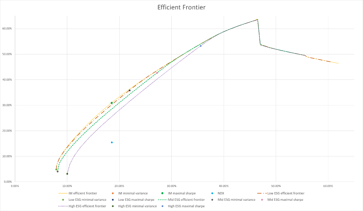
As Figure 1, the step of standard deviation is 0.5% to draw the efficient frontiers. The three thresholds of ESG scenarios are 4.23, 4.95 and 5.67 based on the 3.51 ESG score of the optimal portfolio. It is well-known that theoretically the efficient frontier should look like a parabola with an opening to the right due to the diminishing marginal returns of risk. But that is the case where global stocks are included in the universe. In this research, however, there are only 81 stocks available. So the curve cannot keep smooth all the way. It is inevitable to display a drop at some point, for example, the one at about 47% of standard deviation in Figure 1. Taking a glance at the data will provide explanation to this big drop in return. NVDA has the highest return of 63.6% and a rather high standard deviation of 46.6%. The return of the target portfolio can be controlled smoothly by the weight of NVDA as long as the standard deviation of the target portfolio is below 46.6%. But above that point, higher standard deviation cannot be reached with even 100% of NVDA. Then the GRG method starts to look for stocks with higher standard deviation and sacrifice the high return of NVDA in exchange of higher standard deviation, causing the sudden drop of the efficient frontier. Despite that, the graph looks normal.

The point standing for NDX lies inside all the four frontiers. It means that the target portfolio can beat the market in all the three ESG scenarios over a long term. The four frontiers from outside to inside are IM frontier, low ESG frontier, mid ESG frontier and high ESG frontier. This obviously shows that as the constraint of ESG levels up, the feasible region of the same universe of stocks lessens. But the speed of lessening is quite low. Generally, the four frontiers are close. The biggest gap of return between IM frontier and high ESG frontier is only 10.6% at the minimal variance point of high ESG frontier. And the same gap is 3.44% between IM frontier and mid ESG frontier, 0.79% between IM frontier and low ESG frontier. Another feature depicted in the graph is how the frontiers in different ESG scenarios converge to the IM frontier. When the level of standard deviation is high enough, all the frontiers become the same. The divergence from IM frontier only happens at low standard deviation level. And the level of standard deviation where divergence ends for each frontier is exhibited to be positively correlated with the level of ESG constraint, which is 39.5% for high ESG frontier, 32.5% for mid ESG frontier, 25.5% for low ESG frontier. A possible explanation is that ESG investing lowers the potential volatility in the future. Meanwhile, the return of ESG investing also decreases as a trade-off. The effect may be significant when the required volatility is low. But as the required volatility rises, difference in potential volatility of the portfolio made by ESG constraint become less and less and eventually may be neglected compared to the already high enough volatility at some point.

There is one more unique feature of the low ESG frontier. Unlike the other two, it starts from the same minimal variance point as IM frontier and does not diverge until standard deviation exceeds 8.5%. This shows that ESG investing does not always mean sacrificing potential return. The optimal portfolio does not necessarily have the lowest ESG score. The ESG score of the minimal variance point of IM frontier is 4.62, even higher than the low-ESG threshold of 4.23. Therefore, the low-ESG constraint does not actually take effect at the beginning. This phenomenon does not always happen. In this research, it can be greatly accredited to NVDA. As is mentioned above, NVDA has the highest single stock return. Its standard deviation of 46.60% makes it also the single stock with highest Sharpe ratio. What’s more, it has the second highest ESG score of 6.28. The high Sharpe ratio and high ESG score characteristics make NVDA largely guarantee the high return of target portfolio despite the ESG constraint. It can be inferred that if more stocks in the universe are like NVDA, the frontiers in ESG scenarios will get closer to IM frontier.

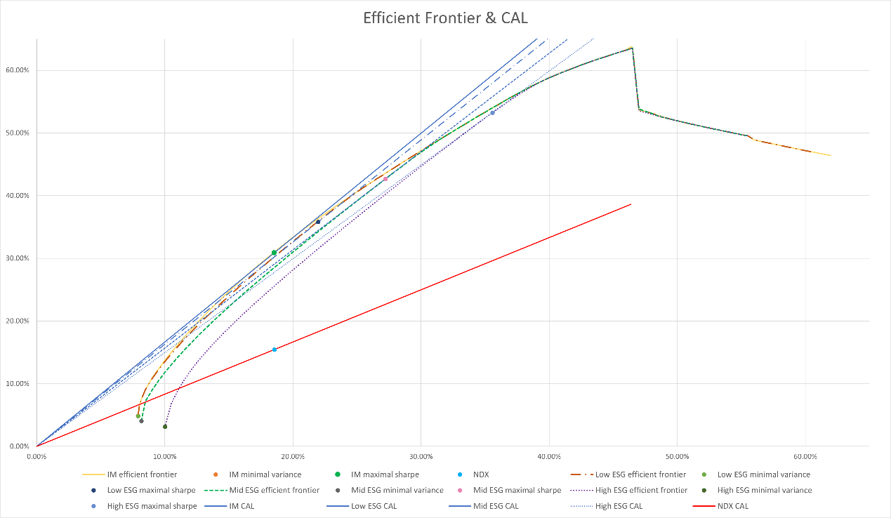
In Figure 2, CALs of each maximal Sharpe ratio portfolio are drawn to reconfirm the effect of ESG constraint. The slopes of blue lines are close, still in the order of ESG level, showing the limited weakening effect of ESG constraint on return. The red line, however, has a fairly smaller slope, proving that ESG investing is strong enough to beat the market index.

3.2. Dynamic analysis

Static analysis above focuses on long-term effect of ESG constraints. In this part, annual returns of modified portfolios in each scenario are calculated to study the short-term performance of ESG investing.

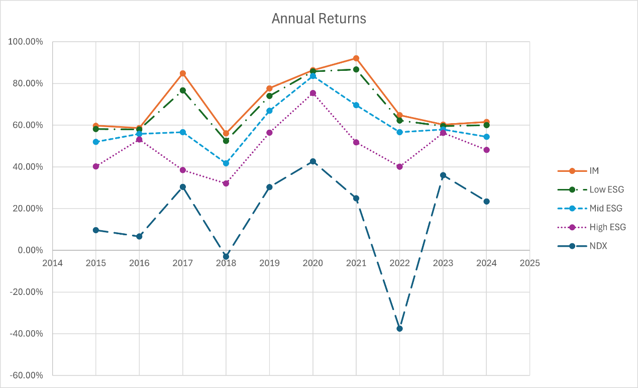
As Figure 3, the dynamic analysis result basically matches with static analysis. The performances of different modified portfolios are, though extremely close in some specific years, strictly ranking in the order of ESG constraint level. And the excess of return over the market index is considerable.

From the trends of the last decade, modified portfolios apparently have steadier performances than the market index, especially in 2018 and 2022 when the stock market plummeted. For clear comparison, table 1 below shows the standard deviation of the annual returns.

The modified portfolios have even smaller standard deviation than the optimal portfolio of IM, suggesting that the introduction of ESG constraint probably does remove some kind of uncertainty and smooth the return, which is consistent with the explanation above mentioned in static analysis. This influence is not linear given that both Low-ESG scenario and High-ESG scenario have higher standard deviation than Mid-ESG scenario. After all, keep pursuing the higher ESG score will end up holding 100% of the single stock with the highest ESG score, whose idiosyncratic risk is not diversified at all.

4. Conclusion

As ESG investing develops from some charitable activity to sustainable wisdom, investors need to understand the influences it has on practical investment. This article uses empirical research to prove that portfolio with ESG constraints can easily outperform the market index while slightly underperform the theoretical optimal model. This not only provides supportive evidence of the benefit of ESG factors but suggests investors a possible easy measure for evaluating the stability of their portfolios. There is also a preliminary finding that ESG constraints may have some non-linear effect of smoothing the return of portfolios, which could be worthy of further study.

There are some main limitations of this research. First, the subject market NASDAQ has features of high volatility and concentration on high-tech sector. Confined to the length and computation, this article does not expand the subject to NYSE to use a larger number of stocks as universe and S&P 500 Index as benchmark, which can be done in future research. Second, the quality and intactness of ESG score data are not satisfying enough. This has been a generally acknowledged problem of ESG factors. Different indicator system and evaluation criteria weaken the objectivity of ESG scores. And companies’ limited disclosure of their ESG related information without mandatory regulations makes the data incomplete for some years. As ESG investing develops, it is foreseeable that the ESG score data will be more and more precise and complete. Then the direction of research can even be focused on the three ESG pillar scores to distinguish the influence of environmental, social and governance factors separately.

References

[1]. Kuzmina, J., & Lindemane, M. (2017). Esg Investing: New Challenges and New Opportunities. Journal of business management, (14).
[2]. Eccles, N. S., & Viviers, S. (2011). The origins and meanings of names describing investment practices that integrate a consideration of ESG issues in the academic literature. Journal of business ethics, 104(3), 389-402.
[3]. Heinkel, R., Kraus, A., & Zechner, J. (2001). The effect of green investment on corporate behavior. Journal of financial and quantitative analysis, 36(4), 431-449.
[4]. Barko, T., Cremers, M., & Renneboog, L. (2022). Shareholder engagement on environmental, social, and governance performance. Journal of Business Ethics, 180(2), 777-812.
[5]. Drei, A., Le Guenedal, T., Lepetit, F., Mortier, V., Roncalli, T., & Sekine, T. (2019). ESG investing in recent years: New insights from old challenges. Available at SSRN 3683469.
[6]. Wang, Z., Zhang, Y., & Li, X. (2018). An empirical study on ESG investment portfolios under parametric quadratic programming compared with stock market indices. Proceedings of the 20th Annual Conference of China Management Science, 579–584.
[7]. Markowitz, H. M. (1952) Portfolio Selection. Journal of Finance, 7(1), 77-91.
[8]. Sharpe, W. F. (1964). Capital asset prices: A theory of market equilibrium under conditions of risk. The journal of finance, 19(3), 425-442.
[9]. Lasdon, L. S., Waren, A. D., Jain, A., & Ratner, M. (1978). Design and testing of a generalized reduced gradient code for nonlinear programming. ACM Transactions on Mathematical Software (TOMS), 4(1), 34-50.
[10]. Chapra, S. C., & Canale, R. P. (2011). Numerical methods for engineers (Vol. 1221). New York: Mcgraw-hill.
Cite this article
Zhang,X. (2025). An Empirical Study on Performance Comparison Between ESG Portfolio and Stock Market Index with Generalized Reduced Gradient Method. Advances in Economics, Management and Political Sciences,218,38-44.
Data availability
The datasets used and/or analyzed during the current study will be available from the authors upon reasonable request.
Disclaimer/Publisher's Note
The statements, opinions and data contained in all publications are solely those of the individual author(s) and contributor(s) and not of EWA Publishing and/or the editor(s). EWA Publishing and/or the editor(s) disclaim responsibility for any injury to people or property resulting from any ideas, methods, instructions or products referred to in the content.
About volume
Volume title: Proceedings of ICEMGD 2025 Symposium: Resilient Business Strategies in Global Markets
© 2024 by the author(s). Licensee EWA Publishing, Oxford, UK. This article is an open access article distributed under the terms and
conditions of the Creative Commons Attribution (CC BY) license. Authors who
publish this series agree to the following terms:
1. Authors retain copyright and grant the series right of first publication with the work simultaneously licensed under a Creative Commons
Attribution License that allows others to share the work with an acknowledgment of the work's authorship and initial publication in this
series.
2. Authors are able to enter into separate, additional contractual arrangements for the non-exclusive distribution of the series's published
version of the work (e.g., post it to an institutional repository or publish it in a book), with an acknowledgment of its initial
publication in this series.
3. Authors are permitted and encouraged to post their work online (e.g., in institutional repositories or on their website) prior to and
during the submission process, as it can lead to productive exchanges, as well as earlier and greater citation of published work (See
Open access policy for details).