1. Introduction

The bond market is one of the important platforms for corporate financing in China, and its stable operation is crucial to the healthy development of the entire capital market. Since the "rigid payment" (i.e., the implicit guarantee of principal and interest repayment) was broken, bond default incidents have occurred frequently. The wholesale and retail industry is one of the industries with a high incidence of defaults. As a key part of the modern commercial and trade circulation system, this industry urgently needs to establish an efficient default early warning mechanism. With the development of big data and artificial intelligence, machine learning methods have provided a new path for default prediction. Based on existing research, this study constructs a serial RF-BP model and verifies it with the case of Gome Electrical Appliances, which has suffered substantive defaults. The purpose is to improve the early warning capability under small-sample conditions and supplement existing research on feature selection and model fusion.

2. Literature review

2.1. Research on influencing factors of corporate bond defaults

Bond defaults are jointly affected by the macro-environment, internal corporate characteristics, and governance mechanisms. From a macro perspective, GDP fluctuations and monetary policy adjustments will change the corporate financing environment and affect debt-servicing capacity. Li Yachao et al. pointed out that the impact of corporate integration strategies on default risk varies in different stages of the economic cycle [1]. Among internal factors, financial leverage, asset-liability ratio, and asset liquidity are particularly critical. Yang Jinqiang et al. found that a decline in asset liquidity directly exacerbates default risk [2]; Sun Lin et al. emphasized that high leverage weakens the competitiveness of core businesses, and long-term debt is more likely to accumulate risks [3]. In terms of governance mechanisms, Dou Chao et al. argued that independent directors with a macro-background can reduce defaults [4]; Qin Jidong et al. pointed out that the absence of an actual controller may intensify agency conflicts and financing constraints [5]; Pan Yalan believed that employee stock ownership plans can alleviate agency problems and reduce the possibility of defaults [6].

2.2. Application of machine learning in default prediction

Machine learning outperforms traditional methods in default prediction due to its ability to capture nonlinear relationships and process high-dimensional data. Wang Yulong et al. and Park D. both confirmed that RF has outstanding prediction performance [7]. Jiang Fuwei et al. integrated macro and micro variables and used 10 machine learning algorithms, finding that nonlinear models (e.g., AdaBoost) have better prediction effects [8]. Hu Yalan used Support Vector Machine (SVM) to identify the credit risk of commercial and retail enterprises [9]. L Yuyong et al. applied temporal deep learning and Graph Neural Network (GNN) combined with market information to improve prediction effectiveness [10]. Gao Yan and Yang Guijun et al. combined Principal Component Analysis (PCA) with BP Neural Network, achieving high accuracy; the latter improved data quality through methods such as Benford's Law [11,12]. Li Chenggang et al. integrated text analysis with BP Neural Network, which performed better than SVM in large samples [13].

2.3. Literature commentary

Existing studies have extensively explored the influencing factors and prediction methods of bond defaults, but there is no consensus on the performance of machine learning models. The BP Neural Network performs well when the sample size is above medium, financial data is complete, and nonlinearity is significant, especially in fields such as private enterprises and local government bonds. However, it still has problems of overfitting and insufficient interpretability. Therefore, this study intends to combine the BP Neural Network with RF for feature selection, construct a serial fusion model, and conduct case verification.

3. Construction of the RF-BP neural network default risk early warning model

3.1. Initial selection of samples and indicators

3.1.1. Sample and time scope

To ensure consistency between prediction timeliness and data availability, this study uses the public information of enterprises in the complete fiscal year (year t) before the occurrence of defaults as independent variables to predict whether substantive defaults will occur in year t+1. Since the number of bond-defaulting enterprises in the same industry is limited, enterprises in the same industry with similar asset scales and indicator characteristics are selected, and samples with missing data are excluded. Finally, 95 samples are obtained, including 19 defaulting enterprises and 76 non-defaulting enterprises. For non-default samples, the same observation period (year t) as that of defaulting enterprises is used; if the default incident occurs earlier than the annual report disclosure, the most recent year with complete disclosure is used and marked as a cross-year observation. To avoid look-ahead bias, a "90-day lag for availability" rule is set for annual report data; defaulting enterprises are defined as samples that failed to fully repay principal or interest on schedule, underwent substantive maturity extension, or were formally identified as defaulting by rating agencies. To address the class imbalance problem, the ADASYN oversampling algorithm is used to balance the training set, while the validation set and test set maintain their original distribution to ensure the objectivity of evaluation and consistency of standards.

3.1.2. Initial selection of indicators

Constructing a scientific and reasonable financial risk early warning indicator system is important for improving the accuracy of prediction models. In the initial indicator selection stage, this study focuses on key variables that can effectively reflect the financial risk status of enterprises. Combined with the characteristics of the wholesale and retail industry (which emphasizes operational efficiency and capital liquidity) and existing research, and considering the risk formation mechanism of this industry, a financial risk early warning indicator system suitable for the industry is finally established. This system includes five major types of indicators: debt-servicing capacity, development capacity, operating capacity, profitability, and cash flow, as shown in Table 1.

3.2. Indicator selection by random forest

RF conducts indicator selection by weighted accumulation and ranking of the "stable marginal contribution of features to purity or prediction performance" across multiple trees, multiple random perturbations, and multiple-fold cross-validation. Using cumulative contribution or stability as the threshold, an interpretable feature subset that balances model performance and feature simplicity is obtained. To obtain an indicator set that is "highly discriminative, moderately dimensional, and clearly defined" before constructing the bond default early warning model, RF is used for feature selection.

3.2.1. Data preprocessing

First, missing values and outliers in the collected data are handled: missing values are imputed with the median of numerical columns, and 1%/99% quantile winsorization is applied to reduce the impact of extreme values. After handling missing values and extreme values, Z-score standardization is uniformly performed on the data. After the above processing, 95 data samples (19 default samples and 76 non-default samples) are used for RF feature importance selection, covering 19 indicators.

3.2.2. Parameter setting

In RF feature selection, the overall parameter setting principle is to prioritize the stability of feature importance ranking under the conditions of small sample size and strong correlation among financial indicators, while controlling overfitting and balancing efficiency. Therefore, a large forest scale, moderate randomization, and stratified cross-validation are adopted to unify the evaluation standard. The main parameter settings are shown in Table 2.

3.2.3. Results of RF feature selection

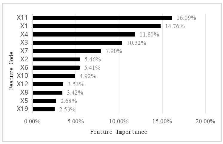
The training results show that the RF model has an AUC (Area Under the ROC Curve) value of 0.9875 and a standard deviation of 0.0105, indicating stable model performance and small fluctuations in prediction results. From the feature importance ranking, key indicators show an obvious concentrated trend at the top, indicating that a small number of core variables provide the main discriminative power. To improve the generalization ability of the small-sample neural network model and control the risk of overfitting, 12 key indicators are finally determined based on the screening criterion of "cumulative contribution ≥ 90%", as shown in Figure 1.

3.3. Construction of the BP neural network early warning model

In this study, for the bond default early warning of the wholesale and retail industry, the features screened by RF (with cumulative contribution ≥ 90%) are used as inputs. Specifically, 12-dimensional standardized numerical features are used, and a feedforward BP Neural Network is adopted to predict the default probability. All standardization parameters and sample balancing in this study are only fitted on the training set and applied to the corresponding validation set; the test set always maintains its original distribution.

3.3.1. Input layer design

The input layer nodes of the neural network correspond to the 12 indicators screened by RF (with cumulative contribution ≥ 90%). Considering class imbalance, ADASYN oversampling is only applied to the minority class in the training set to reduce the impact of data imbalance. The validation set and test set maintain their original distribution without oversampling to ensure an objective evaluation standard. Missing values and outliers have been identified and handled in the data preprocessing stage.

3.3.2. Hidden layer design

The hidden layer adopts a two-layer fully connected structure: the first layer is moderately expanded to 24 nodes (twice the input dimension of 12), facilitating the expansion of multiple nonlinear transformations from the original features; the second layer is reduced to 12 nodes, forming a bottleneck structure. This structure compresses the representation while maintaining representational ability, naturally achieving dimensionality reduction and overfitting suppression. Among the 5-fold cross-validation comparisons of multiple candidate structures, the (24, 12) structure shows more robust performance in terms of AUC, PR-AUC (Precision-Recall AUC), KS (Kolmogorov-Smirnov) statistic, and convergence speed. Although further deepening or widening the structure can improve training fitting, it brings limited gains in external validation and is more prone to overfitting. The ReLU (Rectified Linear Unit) activation function is used, with the formula as follows:

$$$ \begin{array}{c}ReLU\left(x\right)=max(0,x)\end{array}$$$(1)

This activation function has the advantages of stable gradients, fast convergence, and low susceptibility to saturation, making it suitable for the medium-scale task in this study. To suppress overfitting, L2 regularization is applied to the weights; the Adam optimizer is used, and an early stopping strategy is enabled—training stops if there is no improvement in validation indicators for 20 consecutive epochs. The parameter scale of this structure is approximately 625, which matches the sample size and feature dimension, achieving a good balance between expressive ability and overfitting risk.

3.3.3. Output layer design

In the BP Neural Network model, the structure of the output layer is determined by the task objective. For binary classification prediction tasks (default vs. non-default), the number of output layer units is usually set to 1. This unit outputs a probability value between 0 and 1, representing the probability that the sample is classified as default. Through training, the model continuously adjusts weight and bias parameters, mapping the input features to a probability score through nonlinear transformations in the hidden layer. The Sigmoid activation function is used in the output layer to ensure the output value falls within the probability range, with the formula as follows:

$$$ \begin{array}{c}\sigma \left(x\right)=\frac{1}{1+{\mathrm{e}}^{-\mathrm{x}}}\end{array}$$$(2)

3.3.4. Threshold setting

Threshold selection is crucial for default prediction models. Using 0.5 directly as the threshold may fail to balance recall and precision, especially in unbalanced data, where the threshold often needs to be adjusted according to requirements. In the field of risk prediction, the maximum KS statistic is usually used to select the optimal classification threshold. The optimal threshold is determined based on the maximum KS value of the training set probability curve, and then this threshold is used to classify samples into default or non-default. Determining the threshold based on the maximum KS value allows selecting a more appropriate classification boundary while fully considering discriminative power, thereby improving the model's prediction performance and practical application effect.

3.4. Training results

In this model evaluation, the results on both the training set and test set show that the model has strong prediction ability. On the training set, the model performs well in multiple indicators including Accuracy, Recall, Precision, and F1-Score, indicating good fitting effect on the training data and effective identification of default and non-default samples. On the test set, the model's indicators are close to those on the training set, indicating strong generalization ability and good adaptability to unknown data, as shown in Table 3.

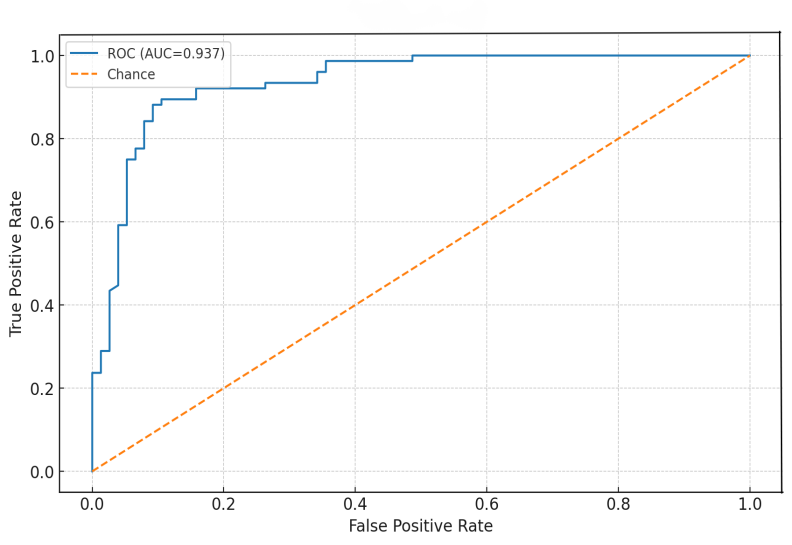
First, RF denoises financial indicators with high correlation; then, the BP Neural Network models nonlinear boundaries and interactive relationships with a simplified structure. This structural design enables the model to balance robustness and expressive ability in small to medium-sized samples. The ROC Curve (Receiver Operating Characteristic Curve) illustrates the model's performance, where the x-axis represents the False Positive Rate (FPR) and the y-axis represents the True Positive Rate (TPR). The upper curve in the figure reflects the model's classification performance under different thresholds, while the lower dashed line represents the benchmark level of a random classifier. The model's AUC reaches 0.937, indicating that its ability to distinguish between positive and negative samples is significantly better than that of random classification, demonstrating strong accuracy in default identification (see Figure 2).

4. Case overview

Gome Electrical Appliances Co., Ltd. was once one of the leading enterprises in China's home appliance retail industry. Founded by the legendary entrepreneur Huang Guangyu, this retail giant, headquartered in Beijing, rapidly expanded its business footprint from Beijing to the entire country in its early stage. Adopting a chain operation model, the company mainly sold home appliances, electronic products, digital products, and household items, building a vast retail network. In recent years, affected by fierce market competition, the impact of online business, and corporate governance issues, this established home appliance retail enterprise has shown poor performance, maintained a high debt scale, and faced significant financial pressure and operational challenges. It began to experience substantive bond defaults in 2023; in fact, there were obvious signs of bond defaults as early as 2022. The details of its bond defaults are shown in Table 4.

5. Case analysis based on the RF-BP neural network default early warning model

In this study, the historical data of year t is introduced into the prediction model to predict the bond default risk of year t+1. In practical verification, the 12-dimensional financial data of the case enterprise (Gome Electrical Appliances) from 2018 to 2023 are selected as samples to predict Gome's default status from 2019 to 2024. The prediction results are compared with the actual status of the corresponding years to evaluate the prediction accuracy of the model. The prediction results are shown in Table 5.

The default probabilities predicted by the model for 2023 and 2024 are as high as 98.74% and 98.67%, respectively, both falling in the extremely high-risk range. This discrimination result is consistent with the actual default facts. From the perspective of early warning timeliness, although the predicted probability in 2022 was 94.44%, which was regarded as a "false positive" under strict thresholds, the enterprise suffered substantive default one year after this signal appeared. Moreover, the case enterprise showed deteriorated financial conditions and a downgraded credit rating in 2022, indicating that the model actually provided effective early risk warning and demonstrated forward-looking identification ability for major credit risks. The predicted probabilities from 2019 to 2021 were always far below the default threshold, consistent with the actual status, which shows that the model also has good stability and anti-interference ability in the low-risk stage.

6. Conclusion

Aiming at the limitations of default early warning models under high-dimensional indicators and unbalanced samples, this study constructs a serial fusion model combining RF and BP Neural Network. Based on the characteristic indicator system of the wholesale and retail industry, the model first uses RF for key feature selection, then applies the BP Neural Network for nonlinear fitting. It shows good stability and prediction performance under small to medium-sized samples. The experimental results show that the model achieves good results in both the training and testing phases, and successfully realizes the early identification of Gome Electrical Appliances' default risk, demonstrating high practical application value.

References

[1]. Li, Y. C., & Bao, X. J. (2020). Integration degree, macroeconomic fluctuations and corporate debt default. Modern Finance and Economics (Journal of Tianjin University of Finance and Economics), 40(08), 73-87. https: //doi.org/10.19559/j.cnki.12-1387.2020.08.006
[2]. Yang, J. Q., Lin, C. P., & Hu, T. (2022). Asset liquidity, government bailout intensity and corporate default risk. Systems Engineering-Theory & Practice, 42(09), 2333-2349.
[3]. Sun, L., & Sun, J. (2022). Analysis of influencing factors of listed companies' bond default: A study based on corporate financial leverage and diversified operation. Shanghai Finance, (11), 2-11. https: //doi.org/10.13910/j.cnki.shjr.2022.11.001
[4]. Dou, C., Yang, X., Liu, W., et al. (2022). Independent directors' macro perspective and corporate debt default. Accounting Research, (07), 58-74.
[5]. Qin, J. D., Deng, D., & Liu, J. W. (2023). No actual controller and corporate debt default risk. Shanghai Finance, (12), 3-18. https: //doi.org/10.13910/j.cnki.shjr.2023.12.001
[6]. Pan, Y. L., & Xu, A. M. (2023). Can employee stock ownership plans inhibit corporate debt default risk? Journal of Hangzhou Dianzi University (Social Sciences Edition), 19(02), 25-33+41. https: //doi.org/10.13954/j.cnki.hduss.2023.02.004
[7]. Wang, Y. L., Zhou, L., & Zhang, D. F. (2022). Corporate debt default risk prediction: From the perspective of machine learning. Fiscal Science, (06), 62-74. https: //doi.org/10.19477/j.cnki.10-1368/f.2022.06.010
[8]. Jiang, F. W., Lin, Y. H., & Ma, T. (2023). Corporate bond default risk under the background of "breaking rigid payment": Machine learning early warning and economic mechanism exploration. Journal of Financial Research, (10), 85-103.
[9]. Hu, Y. L. (2024). Early warning and prevention strategies of bond default risk for commercial circulation enterprises: Analysis based on support vector machine algorithm. Journal of Commercial Economics, (18), 164-167.
[10]. Li, Y., Wang, Z., & Ma, F. (2023). Bond Default Prediction with Temporal Graph Convolutional Neural Network and Weakly Supervised Learning. Procedia Computer Science, 221, 1376-1385.
[11]. Gao, Y., Du, Y., & Zeng, S. (2023). Research on financial risk early warning of manufacturing enterprises based on BP neural network. Friends of Accounting, (01), 62-70.
[12]. Yang, G. J., Du, F., & Jia, X. L. (2022). Financial risk early warning model of BP neural network based on first and last quality factors. Statistics & Decision, 38(03), 166-171. https: //doi.org/10.13546/j.cnki.tjyjc.2022.03.031
[13]. Li, C. G., Jia, H. Y., Zhao, G. H., et al. (2023). Credit risk early warning of listed companies based on information disclosure text: Empirical evidence from management discussion and analysis in Chinese annual reports. Chinese Journal of Management Science, 31(02), 18-29. https: //doi.org/10.16381/j.cnki.issn1003-207x.2020.2263
Cite this article
Zhu,X. (2025). Early Warning of Bond Defaults in Wholesale and Retail Enterprises: An Integrated Random Forest–BP Neural Network Approach. Advances in Economics, Management and Political Sciences,227,42-51.
Data availability
The datasets used and/or analyzed during the current study will be available from the authors upon reasonable request.
Disclaimer/Publisher's Note
The statements, opinions and data contained in all publications are solely those of the individual author(s) and contributor(s) and not of EWA Publishing and/or the editor(s). EWA Publishing and/or the editor(s) disclaim responsibility for any injury to people or property resulting from any ideas, methods, instructions or products referred to in the content.
About volume
Volume title: Proceedings of the 9th International Conference on Economic Management and Green Development
© 2024 by the author(s). Licensee EWA Publishing, Oxford, UK. This article is an open access article distributed under the terms and
conditions of the Creative Commons Attribution (CC BY) license. Authors who
publish this series agree to the following terms:
1. Authors retain copyright and grant the series right of first publication with the work simultaneously licensed under a Creative Commons
Attribution License that allows others to share the work with an acknowledgment of the work's authorship and initial publication in this
series.
2. Authors are able to enter into separate, additional contractual arrangements for the non-exclusive distribution of the series's published
version of the work (e.g., post it to an institutional repository or publish it in a book), with an acknowledgment of its initial
publication in this series.
3. Authors are permitted and encouraged to post their work online (e.g., in institutional repositories or on their website) prior to and
during the submission process, as it can lead to productive exchanges, as well as earlier and greater citation of published work (See
Open access policy for details).