1.  Introduction

Sustainability is being taken into account more and more when allocating capital, raising new concerns about the relationship between environmental goals, risk, and expected returns. Theory suggests that "green" tilts can impact required returns through clientele and risk channels, and it incorporates non-pecuniary preferences into equilibrium [1]. Empirically, carbon-transition risk seems to be priced: as investor interest in decarbonisation and policy pressure increase, companies with higher emissions experience different expected-return patterns [2]. Climate-news indices also demonstrate how information shocks about physical and transitional risks affect asset prices and produce dynamics of state-contingent returns [3].

Measurement noise in vendor ESG ratings, which frequently differ significantly, presents an implementation challenge [4]. In practice, downside-sensitive methods (such as mean-CVaR and robust variants) offer manageable means of handling asymmetric losses and model uncertainty when building a portfolio [5-6]. Evidence from Australia shows that ESG integration changes sector exposures and that relative performance varies depending on the design and regime [7]. The Australian market is a suitable testbed for transition-risk analysis due to its composition, which is primarily composed of resources and financials, its material emissions intensity, and the availability of auditable firm-level disclosures. These findings drive a data-driven study conducted in Australia that uses official data sources (prices [8-18], risk-free rates [19], constituents [20], emissions disclosures [21], and climate-risk indices [22]) and local large-cap stocks to quantify risk–return trade-offs under climate conditions and emphasise auditable reported emissions.

This study examines how a portfolio-level carbon intensity cap affects efficiency and tail behaviour under varying climate conditions, as well as whether reported corporate emissions contribute to the explanation of large-cap Australian equity risks. The analysis provides policy-relevant evidence for ESG-aware allocation in the Australian context by (i) linking firm-level emissions to risk diagnostics, (ii) evaluating the efficiency cost of decarbonisation along a mean–CVaR frontier, and (iii) assessing state-contingent performance under transition and physical climate-risk regimes, using reported emissions in place of ratings [1–7].

2. Literature review

2.1. Sustainable investing and equilibrium implications

Sustainability preferences are being directly incorporated into market equilibrium by an increasing amount of research. Pricing in these environments takes into account both cash-flow risk and investor clientele effects, suggesting that when capital moves towards "green" assets, expected returns may tilt [1]. This framework offers a standard for determining whether risk exposures or non-pecuniary demand cause ESG-tilted portfolios to generate varying risk-adjusted returns.

2.2. Carbon-transition risk in asset prices

Evidence from around the world suggests that transition risk associated with carbon exposures is priced: as investor and policy attention to decarbonisation increases, companies with higher carbon intensity emissions command varying expected returns [2]. Both cash flow (policy/technological shocks) and discount rate (risk premia) serve as the channel. This encourages the mapping of emissions from Australian issuers to equity risk, which is subsequently accomplished using the portfolio-level cap and the beta-emissions diagnostic.

2.3. Climate news indices and state-contingent behaviour

To monitor the volume and tone of information flows about climate change, text-based climate news metrics have been created. Hedging strategies around climate news shocks are made possible by these indices, which differentiate transition from physical risk and explain time-variation in returns [3]. The Australian evidence is linked to this state-contingent pricing literature through the use of monthly transition-risk (TRI) and physical-risk (PRI) indices as regime variables in Section 4.

2.4. ESG data frictions and the case for direct emissions

Investors face measurement risk because ESG ratings frequently vary significantly amongst providers [4]. The current study avoids this ambiguity by using reported corporate emissions instead of vendor ratings, which is in line with suggestions to implement ESG policy in portfolios while working with auditable, single-metric constraints.

2.5. Portfolio construction with downside control and robustness

A large body of research examines mean-CVaR and robust formulations for managing model uncertainty and asymmetric risk in portfolio design [5–6]. The sensitivity analysis in Section 4 adopts the robust-optimisation mindset by sweeping the emissions cap and analysing the stability of frontier outcomes, whereas the empirical results here emphasise mean-variance for transparency and data parsimony.

2.6. ESG in the Australian equity market

According to data for Australia, ESG integration can alter sector exposures, and implementation decisions and market conditions affect relative performance [7]. This is consistent with the state-contingent performance and sectoral re-allocation for major ASX constituents reported in Section 4.

In relation to the aforementioned strands, this study (i) assesses state-contingent performance under transition vs. physical climate regimes, (ii) applies a portfolio-level emissions cap to quantify the efficiency cost of decarbonisation, and (iii) relates firm-level emissions to cross-sectional risk diagnostics. The emphasis on reported emissions and Australia offers incremental evidence that is pertinent to policy.

3. Methodology

3.1. Study design

The two interconnected steps of the empirical workflow are (i) asset-pricing diagnostics to identify market and climate exposures (Eq. (1)); and (ii) portfolio optimisation with an explicit carbon-intensity cap at the portfolio level, assessed on a common scenario basis with embedded climate stresses (Eq. (2) with Eqs. (3) – (4), and Eq. (5)). To ensure that conclusions come from structured comparisons rather than a single specification, each option is read against a natural contrast (unconstrained vs. constrained, variance vs. CVaR, baseline vs. shocked regimes).

3.2. Data and sample

The Reserve Bank of Australia cash rate is used to convert monthly total returns (dividends reinvested) into excess returns [19]. The carbon-intensity cap at the portfolio level is anchored by reported Scope 1–2 emissions from the Clean Energy Regulator [21]. In line with climate-news and transition measures, climate information employs a transition-risk proxy [2-3,22]. The S&P/ASX 200 is kept for reference purposes, and the investable set is a representative ten-name ASX large-cap subset covering both higher- and lower-emission sectors. The compiled official series is followed for prices and constituents [8]. The baseline period (monthly) is 2016–2024. The representative ten-name subset includes comparatively lower-carbon financials/ healthcare/ consumer/ tech (CBA, WBC, CSL, WOW, WES, XRO) and higher-carbon resources/ energy (BHP, RIO, WDS, S32) in order to fully express the asset universe [20–21]. In Section 4, climate risk indices are kept for scenario conditioning [22].

3.3. Exposure estimation

As in Eq. (1), rolling 36-month regressions of excess returns on the market and climate factors are used to estimate firm-level sensitivities, with standard errors that are consistent with Newey-West heteroskedasticity and autocorrelation. Test statistics are adjusted for serial correlation and heteroskedasticity, which are common in monthly return residuals. In Section 3.5, the mapping of climate shocks and the portfolio carbon constraint are motivated by the cross-section of climate betas, which is read for monotone association with reported emissions.

$$ \mathrm{r}\mathrm{i},\mathrm{t}\mathrm{ }-\mathrm{ }\mathrm{r}\mathrm{f},\mathrm{t}\mathrm{ }=\mathrm{ }\mathrm{\alpha }\mathrm{i}\mathrm{ }+\mathrm{ }\mathrm{\beta }\mathrm{m},\mathrm{i}·\mathrm{M}\mathrm{K}\mathrm{T}\mathrm{t}\mathrm{ }+\mathrm{ }\mathrm{\beta }\mathrm{c},\mathrm{i}·\mathrm{C}\mathrm{L}\mathrm{M}\mathrm{t}\mathrm{ }+\mathrm{ }\mathrm{\epsilon }\mathrm{i},\mathrm{t}$$(1)

3.4. Portfolio optimisation and frontier evaluation

Portfolios are fully invested and long-only. By solving the mean–CVaR programme in Eq. (2), subject to Eqs. (3) – (4), the efficient set is traced over a grid of target returns. Non-negativity, full investment, and a portfolio carbon intensity cap are among the constraints; sector bandwidths are used where necessary to prevent concentration. Targeting tail losses while maintaining implementation tractability is the goal of the mean–CVaR objective [5-6]. Along the whole frontier, trade-offs are interpreted, emphasising areas where costs become convex as the cap tightens and where decarbonisation is almost free at low-to-moderate stringency. For each target return, constrained and unconstrained solutions are read side-by-side on the common scenario base to keep efficiency and tail behaviour directly comparable.

$$ \mathrm{m}\mathrm{i}\mathrm{n}\mathrm{w},\mathrm{ }\mathrm{\tau },\mathrm{ }\left\{\mathrm{\xi }\mathrm{s}\right\}\mathrm{ }\mathrm{ }\mathrm{\tau }\mathrm{ }+\mathrm{ }1/\left(\right(1-\mathrm{\alpha })·\mathrm{N})\mathrm{ }·\mathrm{ }\mathrm{\Sigma }\mathrm{s}=1..\mathrm{N}\mathrm{ }\mathrm{\xi }\mathrm{s}$$(2)

$$ \mathrm{\xi }\mathrm{s}\mathrm{ }\ge \mathrm{ }-\mathrm{w}\mathrm{ᵀ}\mathrm{ }\mathrm{r}\left(\mathrm{s}\right)\mathrm{ }-\mathrm{ }\mathrm{\tau };\mathrm{ }\mathrm{ }\mathrm{ }\mathrm{\xi }\mathrm{s}\mathrm{ }\ge \mathrm{ }0;\mathrm{ }\mathrm{ }\mathrm{ }\mathrm{s}\mathrm{ }=\mathrm{ }1,\dots ,\mathrm{N}$$(3)

$$ \mathrm{E}\left[\mathrm{w}\mathrm{ᵀ}\mathrm{ }\mathrm{r}\right]\ge \mathrm{ }\mathrm{\mu }\ast ;\mathrm{ }\mathrm{ }\mathrm{ }1\mathrm{ᵀ}\mathrm{ }\mathrm{w}\mathrm{ }=\mathrm{ }1;\mathrm{ }\mathrm{ }\mathrm{ }\mathrm{w}\mathrm{ }\ge \mathrm{ }0;\mathrm{ }\mathrm{C}\mathrm{a}\mathrm{r}\mathrm{b}\mathrm{o}\mathrm{n}\mathrm{I}\mathrm{n}\mathrm{t}\mathrm{e}\mathrm{n}\mathrm{s}\mathrm{i}\mathrm{t}\mathrm{y}\left(\mathrm{w}\right)\mathrm{ }\le \mathrm{ }\mathrm{C}\ast $$(4)

3.5. Scenario engine and climate shocks

In order to maintain weak stationarity, time dependence, and cross-asset co-movement, risk is assessed using a common scenario base that is produced by a stationary bootstrap of residuals with geometric block lengths. To maintain cross-asset co-movement without assuming i.i.d returns, blocks are sampled jointly across assets. Equation (5) uses the estimated climate exposures to translate climate shocks into asset-level returns. All evaluations use the same scenario base for like-for-like comparisons, and shock magnitudes are defined in Low/Medium/High bands in relation to the empirical dispersion of the climate factor [2-3,22]. A decarbonisation path is achieved by gradually tightening the portfolio carbon-intensity cap while maintaining other settings constant [21]. Two exercises are carried out: (i) transition shocks of Low/Medium/High magnitude with risk-return metrics recalculated on the same scenario set [2-3,22]. Effects are evaluated along the shock ladder and the cap trajectory to emphasise continuity of responses rather than single-point comparisons.

$$ \mathrm{S}\mathrm{h}\mathrm{o}\mathrm{c}\mathrm{k}\mathrm{e}\mathrm{d}\mathrm{R}\mathrm{e}\mathrm{t}\mathrm{u}\mathrm{r}\mathrm{n}\mathrm{i}\left(\mathrm{s}\right)\mathrm{ }=\mathrm{ }\mathrm{B}\mathrm{a}\mathrm{s}\mathrm{e}\mathrm{l}\mathrm{i}\mathrm{n}\mathrm{e}\mathrm{R}\mathrm{e}\mathrm{t}\mathrm{u}\mathrm{r}\mathrm{n}\mathrm{i}\left(\mathrm{s}\right)\mathrm{ }+\mathrm{ }\mathrm{\beta }\mathrm{c},\mathrm{i}\mathrm{ }·\mathrm{ }\mathrm{S}\mathrm{h}\mathrm{o}\mathrm{c}\mathrm{k}\mathrm{C}\mathrm{l}\mathrm{i}\mathrm{m}\mathrm{a}\mathrm{t}\mathrm{e}\left(\mathrm{s}\right)$$(5)

3.6. Robustness and implementation

Sensitivity analyses change the number of scenarios, the rolling-window length for exposure estimation, the cap stringency, and the risk metric (variance versus CVaR) and its confidence level [5-6]. Robustness also takes into account ESG-rating divergence in the Australian context, and the emissions control is tested in absolute and per-revenue forms while staying portfolio-level and linear [4,7]. For Australian large caps, implementation notes (using sector bandwidths, long-only, and full-investment requirements) guarantee that solutions are still actionable [7-8]. Data, model, and regime sensitivity choices are read together to ensure that conclusions hold up to reasonable design variations.

Expected return, volatility, Sharpe ratio, Value-at-Risk, Conditional Value-at-Risk, maximum drawdown, and portfolio emissions are all reported as like-for-like comparisons based on the common scenario base. In order to guarantee that results represent design decisions and state conditions rather than sampling variation, Eqs. (1) – (5) establish a one-to-one relationship between diagnostics, frontiers, and shocks.

4. Results & discussion

4.1. Asset pricing diagnostics for ASX large caps (2016–2024)

4.1.1. CAPM estimates and diagnostics

Before the asset-pricing diagnostics, a summary of the descriptive features of the ten-stock universe specified in Section 3.2 is provided. While alphas are typically small and statistically indistinguishable from zero — with XRO being the lone exception — market betas are positive and highly significant for all firms from 2016 to 2024. Resources display lower R square, which is consistent with commodity-specific drivers, while financials (CBA, WBC) have the highest explanatory power (R squares range is approximately 0.49–0.59), suggesting returns that are more closely tied to market conditions.

Sources: prices [8–18], risk-free [19], constituents [20], emissions [21].

Table 1 demonstrates that: (i) Systematic risk is dominant: sector tilts will move portfolio cyclicality, as shown by sector patterns in β (resources/energy ≥ 1; defensives like CSL, WOW ≥ 1). (ii) Alpha is limited: outside of XRO, abnormal returns do not persist after market risk is taken into account. This further supports the idea that the primary lever for ESG-aware allocation is risk shaping (β, tails). (iii) Resources versus financials: banks are more market-driven, a distinction that will be significant in the event of climate shocks, whereas resources carry more idiosyncratic variation (lower R²).

4.1.2. Risk–emissions visual diagnostics

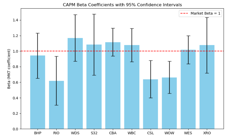
Figure 1 shows that the estimated CAPM Beta coefficients with 95% CIs clearly show sectoral cyclicality. Near-market sensitivity is indicated by BHP's beta, which is near one. Betas for CSL and WOW are less than 0.7, which is in line with defensive traits. In contrast, pro-cyclical exposure is indicated by WDS and S32, which show betas greater than one. These cross-sectional trends suggest that a visual risk-budgeting checklist based on betas and their confidence intervals can assist in identifying inadvertent changes in cyclical tilt when ESG constraints change sector weights. Monthly data for 2016–2024 is used in the estimates, and excess returns are defined in relation to the RBA cash rate target and constituent prices for the chosen ASX names [8]. The ensuing ESG-constrained analyses are supported by reported emissions [21].

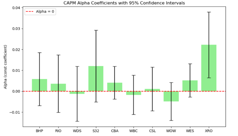
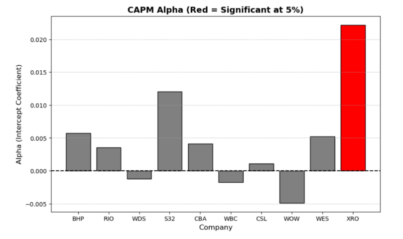
Figures 2 and 3 show that, for the majority of constituents over the period 2016–2024, CAPM alpha estimates with 95% CIs show no persistently abnormal performance: formal tests do not reject a zero intercept at the 5 percent level, and the confidence intervals largely straddle zero. The only exception, with a positive and statistically significant alpha, is XRO. The near-zero alphas for the remaining names suggest that market exposure, rather than stock-specific abnormal performance, is the primary factor capturing cross-sectional return differences. These diagnostics are intended to identify out-of-market adjustment or persistent underperformance. The evidence favours using conservative expected-return assumptions in optimisation and giving risk management and ESG constraints precedence over alpha pursuit when building a portfolio [8].

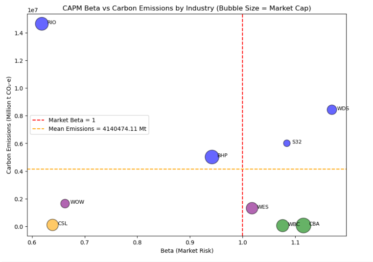
Figure 4 shows a distinct quadrant structure formed by reported emissions and systematic risk (Beta). First, WDS and S32, the first names to bind under portfolio carbon caps, are found in the upper-right quadrant (high Beta, high carbon), which tends to increase portfolio carbon while intensifying market drawdowns [11–12, 21]. Second, as demonstrated by the upper-left quadrant (high carbon, low beta), high emissions do not necessarily indicate high market sensitivity. RIO's position is a reflection of long-cycle demand and commodity structure, which during the sample period reduced beta [10, 21]. Third, CBA and WBC are located in the lower-right quadrant (low carbon, high beta); they have a low ESG footprint but are useful for reducing financed emissions without lowering exposure to growth because of their pro-cyclical exposure [13–14, 21]. Lastly, WOW and CSL, which serve as defensive low-carbon anchors that aid in portfolio stabilisation during shocks, are located in the lower-left quadrant (low carbon, low beta) [15–16, 21].

A layer of market capitalisation that is pertinent to implementation is added by bubble size. While smaller resource firms (like WDS and S32) more frequently combine higher Betas with high emissions, mega-caps like BHP tend to lie close to Beta = 1, suggesting that cap-weighted allocations can moderate risk for a given carbon footprint. Large-cap banks and retailers, on the other hand, offer organic low-carbon alternatives that maintain market exposure (for banks, betas at or above one) without going over the carbon budget when portfolio carbon caps tighten [8, 20-21].

4.1.3. Portfolio implications

Sector tilts and ESG goals are closely related in Australia's market structure. Tightening a carbon intensity cap on a portfolio mechanically changes the cross-sectional distribution of beta and decreases exposure to energy and resources; these changes must be weighed against return goals [8–12, 20–21]. Beta and tail-risk controls serve as the main tools for achieving ESG goals without significantly compromising performance because estimated CAPM alphas are typically insignificant and the practical lever is in risk rather than abnormal return [8, 19, 21]. The contrast between RIO and WDS/S32 along the ESG-constrained frontier supports nuanced carbon constraints—caps and sector-specific bandwidths—rather than blunt exclusions, allowing decarbonisation while maintaining desired market exposure. As a result, high-carbon names should not be treated uniformly for implementation [10–12, 21].

4.2. Portfolio optimisation under a portfolio-level emissions cap

4.2.1. Setup and constraints

For 2016–2024, monthly excess returns are calculated in relation to the RBA cash rate [19]. The S&P/ASX 200 constituent list is compared to the investable universe [20]. A portfolio-level emissions cap is enforced using the Clean Energy Regulator's scope 1-2 emissions for 2023–2024 [21]. These restrictions are then used to re-optimize the same ten ASX names that were defined in Section 3.2.

4.2.2. Minimum-variance corner

The emissions cap lowers portfolio emissions from roughly 14,906,420 to 12,302,950 tonnes CO2-e (a 17–18 percent reduction), while volatility is almost flat (0.0378 to 0.0381) and the expected monthly return is essentially unchanged (-0.008997 vs -0.008959). The Sharpe ratio, calculated using the RBA cash rate, is -0.3043 as opposed to -0.3008; risk-adjusted performance is essentially unchanged. To put it briefly, the cap accomplishes material decarbonisation at the low-risk corner without an efficiency penalty [19, 21].

4.2.3. Efficient frontier: with vs. without the cap

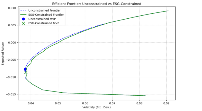
The minimum-variance points are indicated and efficient frontiers are superimposed in Fig.5. Only in the very low-risk region does the ESG-constrained frontier lie marginally below the unconstrained frontier; as target risk increases, the two curves almost coincide. In contrast to banks, retail, and healthcare, which had lower emissions and betas closer to the market, high-carbon miners and energy names combined high emissions with market-or-above betas (see section 4.1). Therefore, at little cost to variance, the cap substitutes lower-emission sectors for a small portion of low-idiosyncratic-risk mining exposure [8, 21].

4.2.4. Sectoral reallocation under the cap

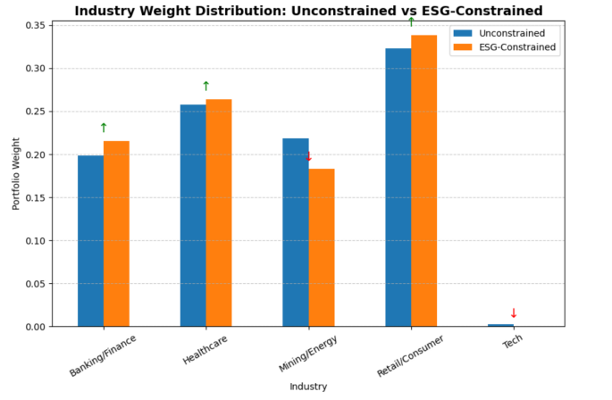
Weights are aggregated by industry in Fig.6. Technology is insignificant at the minimum-variance point; mining and energy decline under the cap, while banking and finance, healthcare, and retail/consumer rise. This mechanism, which is in line with the cross-sectional risk and emissions patterns reported in 4.1 [8, 20-21], is responsible for both the small frontier movement and the large emissions decline.

4.2.5. Sensitivity to the emissions threshold

While the return response is non-linear, ranging from -0.008997 to -0.008951 to -0.009139 per month, with only minor volatility changes (from 0.0378 to 0.0384), tightening the cap from 1.5×10^7 to 1.2×10^7 to 1.0×10^7 tonnes CO2-e reduces portfolio emissions roughly linearly. A practical knee, the 1.2×10^7 setting minimises efficiency costs while securing the majority of the decarbonisation benefit [8, 20-21].

4.2.6. Implementation implications

When combined, the implementation results point to the following conclusions. First, without a quantifiable efficiency penalty, a portfolio-level emissions cap can lower financed emissions by roughly 18 percent at the minimum-variance corner with current CER disclosures [21]. Second, costs are localised: ESG-related efficiency losses concentrate in ultra-low-risk allocations, while the efficient frontiers converge at higher-risk targets (Fig. 5). Third, the mechanism is sectoral: the cap reallocates weight away from energy and high-carbon miners towards banks, retail, and healthcare (Fig. 6), in line with the diagnostics in Section 4.1. Fourth, a cap of roughly 1.2x10^7 tonnes CO2-e is a practical calibration for this ASX sample, achieving the majority of the decarbonisation before return losses accelerate. Lastly, these tilts serve as a link to Section 4.3: using external climate-risk indices puts the portfolio in a position to handle transition-risk shocks that are studied under climate scenarios [22].

4.3. Climate scenario analysis

4.3.1. Time-series properties of climate risk indices

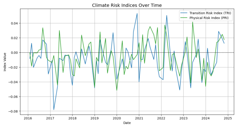
Continue using the earlier data for additional research and analysis. The "Climate Risk Indexes" series is the source of the Transition Risk Index (TRI) and Physical Risk Index (PRI) [22]. TRI/PRI terciles are used to create High, Medium, and Low climate-risk scenarios for the 2016–2024 study period. Both TRI and PRI show noticeable month-to-month variability around zero with sporadic spikes (particularly 2020–2021), as shown in Fig.7. This pattern aligns with the documented episodic bursts of physical risk salience (extreme weather and climate science coverage) and transition news (policy and decarbonisation salience) for these indices [22]. The absence of persistent drift implies that the pressure from climate news is episodic rather than trending, meaning that exposures to portfolios will be most important during spikes rather than quiet times.

The unconstrained minimum-variance solution loads meaningfully on Mining/ Energy and underweights defensives, while the ESG-constrained solution rotates towards Banking/ Finance, Healthcare, and Retail and achieves a double dividend (similar risk/return with materially lower portfolio emissions). Section 4.1 demonstrated that high-emission, resource-intensive names have market betas near or above one and dominate the right-hand side of the beta–emissions scatter. These variations in composition suggest different reactions to physical-risk salience (PRI) and transition-news spikes (TRI).

4.3.2. Portfolio returns by TRI/PRI scenario

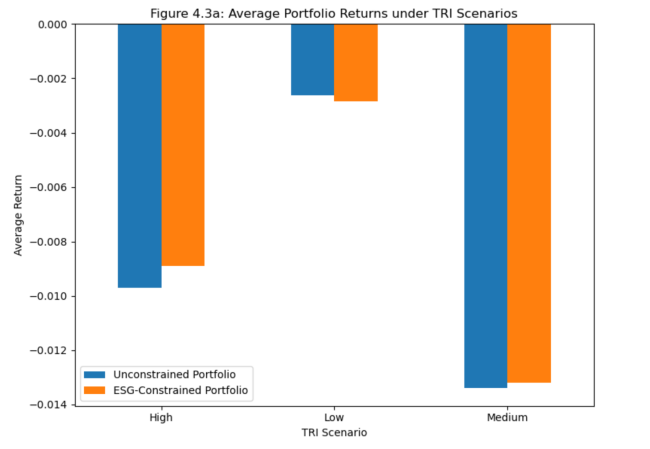
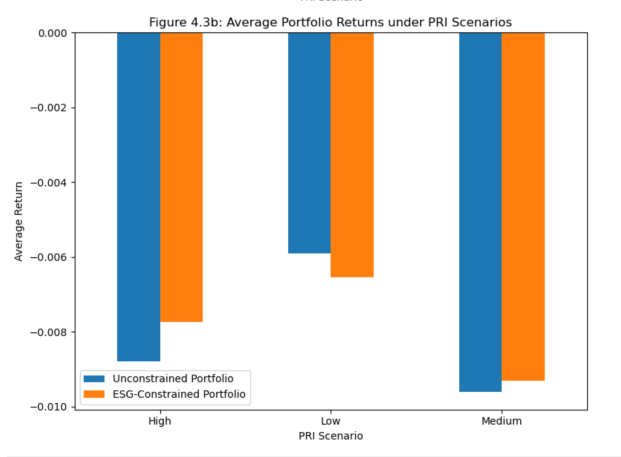
A distinct regime-dependent pattern can be seen in Figures 8 and 9. When transition or physical risk concerns increase, reallocating away from high emitters and towards lower-emission defensives reduces drawdowns, but the improvement is steady but economically modest [22]. In high-risk regimes (TRI=High or PRI=High), the ESG-constrained portfolio shows smaller average losses than the unconstrained allocation. With minor and directionally stable variations, the ESG portfolio typically maintains a slight advantage in average return in moderate-risk regimes. In contrast, the unconstrained portfolio usually outperforms and the performance gap narrows or reverses under low-risk regimes. This is consistent with cyclical recoveries in high-beta, high-emission industries (such as mining and energy) where climate risk is less significant—exactly the industries that are down-weighted by the ESG constraint outlined in Section 4.2.

These trends align with the climate-risk pricing narrative, which holds that transition risk disproportionately penalises high emitters during periods of policy/news intensity, while calm periods allow the cyclicality of carbon-intensive sectors to dominate returns [2,22]. The findings support the conclusion in Section 4.2 that an ESG constraint re-allocates exposure to industries less susceptible to TRI/PRI spikes while maintaining mean-variance efficiency.

4.3.3. Risk and sharpe by scenario

The scenario-conditioned volatility of the two portfolios is almost identical across regimes. Overall, the constraint does not increase risk; the ESG-constrained portfolio shows nearly equal volatility in medium regimes, slightly higher volatility in low regimes, and slightly lower volatility when TRI=High or PRI=High compared to the unconstrained allocation. This pattern is reflected in risk-adjusted results: in High and Medium regimes, the ESG-constrained portfolio has lower negative Sharpe ratios than the unconstrained benchmark (which is consistent with the challenging period of the sample), while in Low regimes, the unconstrained portfolio is slightly better, which is consistent with cyclical recoveries in high-beta, high-emission industries. When combined, these results point to reduced opportunity cost during periods of calm climate and enhanced resilience to negative outcomes during periods of increased climate risk [22].

4.3.4. Synthesis and implications

A state-contingent interpretation is obtained by combining the portfolio reweighting in Section 4.2 with the cross-sectional diagnostics in Section 4.1. The ESG-constrained allocation performs better during spikes in transition or physical risk (TRI/PRI) because it increases weights in banking/finance, healthcare, and retail while mechanically reducing exposure to high-emission, high-beta resource names. This leads to shallower losses in high-risk regimes. The unconstrained portfolio frequently performs slightly better when TRI/PRI is low because high-Beta, high-emission industries typically recover more quickly. As a result, the observed give-back is minimal, happens exactly when climate-risk salience is decreased, and suggests a trade-off that is state-dependent rather than universal [22].

A lower-carbon mean-variance equivalency is also supported by the scenario results. According to CER firm disclosures, the ESG-constrained minimum-variance portfolio provides expected return and volatility that are almost the same as the unconstrained solution, while materially reducing financed emissions in accordance with Section 4.2 [21]. Using Investing.com prices [8-18] and the RBA cash rate as the risk-free series [19], a simple portfolio-level carbon-intensity cap on a representative ASX universe [20] for Australian large caps preserves efficiency, reduces financed emissions, and enhances downside behaviour precisely when climate risk is most prominent in public information (TRI/PRI) [22]. Carbon transition risk is conditional and priced, both theoretically and empirically [2,22].

5. Conclusion

This study combined firm-level exposure diagnostics, mean–CVaR portfolio optimisation, and embedded climate scenarios to investigate whether reported corporate emissions explain risk in Australian equities and how a portfolio-level carbon intensity cap affects efficiency and tail behaviour under changing climate conditions.

The overall outcome is as follows: (i) Asset pricing: climate betas vary with reported emissions and correspond with sector structure; since alphas are limited, risk, not stock-picking, is the controllable margin. (ii) Portfolio optimisation: at higher risk levels, the unconstrained vs. constrained frontiers almost converge, costs are convex as the cap tightens, and an emissions cap achieves material decarbonisation (~18%) with minimal efficiency loss at the minimum-variance corner. (iii) Climate scenarios: constrained portfolios exhibit better tail metrics and shallower losses in High/Medium transition-risk regimes; any give-back in Low regimes is minimal. When climate risk is prominent, mean-variance efficiency is generally maintained while financed emissions decrease and downside resilience increases.

Some of the limitations include the following: the scenario engine abstracts from sudden policy shocks and trading frictions; the universe focuses on large-cap names over a limited window; and the use of Scope 1–2 emissions (supply-chain Scope 3 and physical-risk intensities are not fully captured). Future research should test multi-period rebalancing with costs, benchmark alternative scenario engines and transition pathways, scale the universe and horizon, and include Scope 3 and richer physical-risk metrics.

Last but not least, reported emissions can be used as the operational sustainability control; the cap can be calibrated along a trajectory that acknowledges modest costs at low-to-moderate stringency and accelerates trade-offs beyond that point; climate betas and traditional risk can be monitored to guide rebalancing as transition conditions change; and performance can be evaluated on a common scenario base to separate design effects from sampling noise. The study offers a tractable path for ESG-aware allocation in Australian large caps by establishing a transparent, auditable framework that connects emissions to priced climate exposure and to portfolio outcomes.

References

[1]. Pástor, L., Stambaugh, R. F., Taylor, L. A.: Sustainable investing in equilibrium. Journal of Financial Economics 142(2), 550–571 (2021)
[2]. Bolton, P., Kacperczyk, M.: Global pricing of carbon-transition risk. The Journal of Finance 78(6), 3677-3754 (2023)
[3]. Engle, R. F., Giglio, S., Kelly, B., Lee, H., Stroebel, J.: Hedging climate change news. The Review of Financial Studies 33(3), 1184–1216 (2020)
[4]. Berg, F., Kölbel, J. F., Rigobon, R.: Aggregate confusion: The divergence of ESG ratings. Review of Finance 26(6), 1315–1344 (2022)
[5]. Luan, F., Zhang, W., Liu, Y.: Robust international portfolio optimization with worst-case mean–CVaR. European Journal of Operational Research 303(2), 877–890 (2022)
[6]. Wang, S., Pang, L.-P., Wang, S., Zhang, H.-W.: Distributionally robust mean–CVaR portfolio optimization with cardinality constraint. Journal of the Operations Research Society of China (2023)
[7]. Lee, D. D., Fan, J. H., Wong, V. S. H.: No more excuses! Performance of ESG-integrated portfolios in Australia. Accounting & Finance 61(S1), 2407–2450 (2021)
[8]. S& P/ASX 200 Historical Data, https: //www.investing.com/indices/aus-200-historical-data, last accessed 2025/09/07
[9]. BHP Group Limited Historical Data, https: //www.investing.com/equities/bhp-billiton-limited-historical-data, last accessed 2025/09/07
[10]. Rio Tinto Limited Historical Data, https: //www.investing.com/equities/rio-tinto-limited-historical-data, last accessed 2025/09/07
[11]. Woodside Energy Group Ltd Historical Data, https: //www.investing.com/equities/woodside-petroleum-limited-historical-data, last accessed 2025/09/07
[12]. South32 Limited Historical Data, https: //www.investing.com/equities/south32-ltd-historical-data, last accessed 2025/09/07
[13]. Commonwealth Bank of Australia Historical Data, https: //www.investing.com/equities/commonwealth-bank-of-australia-historical-data, last accessed 2025/09/07
[14]. Westpac Banking Corporation Historical Data, https: //www.investing.com/equities/westpac-banking-corporation-historical-data, last accessed 2025/09/07
[15]. CSL Limited Historical Data, https: //www.investing.com/equities/csl-limited-historical-data, last accessed 2025/09/07
[16]. Woolworths Group Limited Historical Data, https: //www.investing.com/equities/woolworths-limited-historical-data, last accessed 2025/09/07
[17]. Wesfarmers Limited Historical Data, https: //www.investing.com/equities/wesfarmers-limited-historical-data, last accessed 2025/09/07
[18]. Xero Limited Historical Data, https: //www.investing.com/equities/xero-historical-data, last accessed 2025/09/07
[19]. Reserve Bank of Australia, Interest Rates and Yields – Money Market – Monthly – F1.1, https: //www.rba.gov.au/statistics/tables/#interest-rates, last accessed 2025/09/08
[20]. Market Index, S& P/ASX 200 Companies List, https: //www.marketindex.com.au/asx200, last accessed 2025/09/08
[21]. Clean Energy Regulator, Greenhouse and energy information by controlling corporation 2023–24, https: //cer.gov.au/markets/reports-and-data/nger-reporting-data-and-registers/corporate-emissions-and-energy-data-2023-24, last accessed 2025/09/08
[22]. Climate Risk Indexes, https: //www.policyuncertainty.com/Climate_Risk_Indexes.html, last accessed 2025/09/08
Cite this article
Li,Z. (2025). Asset Pricing and Portfolio Optimisation under ESG Constraints: An Actuarial Risk and Climate Scenario Study in Australia. Advances in Economics, Management and Political Sciences,229,1-14.
Data availability
The datasets used and/or analyzed during the current study will be available from the authors upon reasonable request.
Disclaimer/Publisher's Note
The statements, opinions and data contained in all publications are solely those of the individual author(s) and contributor(s) and not of EWA Publishing and/or the editor(s). EWA Publishing and/or the editor(s) disclaim responsibility for any injury to people or property resulting from any ideas, methods, instructions or products referred to in the content.
About volume
Volume title: Proceedings of ICFTBA 2025 Symposium: Data-Driven Decision Making in Business and Economics
© 2024 by the author(s). Licensee EWA Publishing, Oxford, UK. This article is an open access article distributed under the terms and
conditions of the Creative Commons Attribution (CC BY) license. Authors who
publish this series agree to the following terms:
1. Authors retain copyright and grant the series right of first publication with the work simultaneously licensed under a Creative Commons
Attribution License that allows others to share the work with an acknowledgment of the work's authorship and initial publication in this
series.
2. Authors are able to enter into separate, additional contractual arrangements for the non-exclusive distribution of the series's published
version of the work (e.g., post it to an institutional repository or publish it in a book), with an acknowledgment of its initial
publication in this series.
3. Authors are permitted and encouraged to post their work online (e.g., in institutional repositories or on their website) prior to and
during the submission process, as it can lead to productive exchanges, as well as earlier and greater citation of published work (See
Open access policy for details).