


1. Introduction
1.1. Research background
Urban rail investment reshapes effective accessibility and, in turn, the spatial distribution of residential value across metropolitan space. In large, polycentric cities this capitalization is rarely uniform because station catchments differ in built form, travel options, and neighborhood composition. Melbourne offers a pertinent context: it operates Australia’s most extensive suburban rail network alongside the world’s largest tram system, with a heavy-rail grid of 16 lines, roughly 372 km of track, and 218 stations organized radially by a CBD loop; unlike systems that sharply segregate urban and suburban services, Melbourne integrates inner-city, longer-distance, and freight operations within a single network, making it a distinctive case in Oceania (Figure 1). Within this network, the Cranbourne Line runs approximately 50 km southeast from the CBD through mature suburbs, is among the city’s highest-demand corridors (≈160,000 daily passengers), and links major activity nodes such as Chadstone and Monash University, underscoring its policy salience for the 860,060 residents of Southeast Melbourne.
Consistent with corridor-study practice, the empirical lens centers on dwellings within 3 km of the line, where proximity effects are most plausibly observed. Classic hedonic evidence indicates that transit access can be capitalized into rents and prices, establishing an empirical foundation for accessibility–value linkages [1]. Applied corridor studies further document premia associated with rail service and network reach, reinforcing the case for location-specific analysis in urban settings [2]. Meta-evidence from European markets likewise shows that rail accessibility and service quality shape residential valuations in measurable ways [3]. On the methodological side, geographically weighted regression was introduced to explore spatial non-stationarity in relationships that global models may obscure [4]. Comparative work demonstrates that local modeling can recover structure missed by single-coefficient specifications in housing markets [5]. Evidence from Chinese cities shows spatial heterogeneity in implicit prices and the value of local modeling for urban real-estate analysis [6]. Additional applications confirm the usefulness of geographically weighted regression for price–attribute relationships and corridor contexts [7]. Distribution-sensitive approaches reveal that capitalization of station proximity can vary across the price spectrum, underscoring the need to look beyond mean effects [8]. Studies of service timing and rollout show price lifts near commencement followed by distance-decay, highlighting dynamic capitalization patterns around stations [9]. Research in higher-car contexts also finds that station impacts vary with metropolitan structure, emphasizing the importance of local conditions and last-mile integration [10].
1.2. Research gap
Despite a substantial literature on transport capitalization, three limitations reduce portability to Melbourne’s suburban corridors and blunt policy usefulness along multi-station lines like Cranbourne. First, a measurement gap persists because many Australian studies model total sale prices, conflating accessibility premia with lot size, built area, and internal layout; adopting per-square-metre prices restores cross-sectional comparability and sharpens accessibility gradients. Second, a modelling gap arises when global hedonic specifications impose single coefficients that mask spatial non-stationarity in the effects of station proximity, CBD access, and local services; planning decisions are local, so stakeholders need to know not only whether access matters on average but where and by how much along the corridor. Third, a context and covariate gap stems from importing elasticities from compact, low-car cities to a setting with higher car ownership, larger lots, and uneven last-mile conditions; coarse treatment of services and disamenities and reliance on Euclidean rather than network measures further bias inference.
Guided by these issues, the paper asks three questions tailored to corridor decisions: how per-m² prices relate to distance to the nearest station and the CBD conditional on structural and small-area socio-demographics; how service densities (bus stops, schools, hospitals) co-vary with prices net of accessibility; and where along the Cranbourne corridor capitalization is strongest or weakest, indicating station areas where design, last-mile service, or TOD up-zoning would yield the greatest returns. The expected contribution is both analytical and practical: pairing an interpretable OLS benchmark with geographically weighted regression translates heterogeneous effects into policy-readable surfaces while maintaining transparency and replicability in measurement, sample construction, and reporting.
1.3. Fill the gap
To operationalize this agenda, the study assembles a geocoded, dwelling-level dataset for properties within 3 km of the Cranbourne Line and standardizes outcomes to per-m² prices. Property microdata (transaction price and date, bedrooms, bathrooms, on-site parking, age) are linked to SA1 socio-demographics (median age, income, labour-force participation). Accessibility is measured as distance to the nearest rail station, nearest bus stop, and the CBD; local service availability is captured by counts of bus stops, schools, and hospitals within a 5-km buffer. Estimation proceeds on a complete-case sample to preserve a consistent covariate set, with descriptive statistics reported on the broader sample to document distributions and sample flow. Modelling then follows a two-step sequence: a global OLS hedonic specification establishes corridor-wide direction, magnitude, and fit across accessibility, service, structural, and neighbourhood blocks; a geographically weighted regression is subsequently applied to variables exhibiting geographic variability (notably station distance and selected service densities) to produce local coefficient surfaces that reveal where premia intensify or dissipate.
2. Literature table
2.1. Definition
Transit‑Oriented Development (TOD) in this study denotes a development paradigm in which high‑capacity public transport—especially rail—reduces generalized travel costs and restructures urban form around station areas, such that accessibility gains are capitalized into nearby land and housing markets; the node–place perspective clarifies how station functions and surrounding land uses co‑evolve under this logic [11]. Planning instruments and rail plans can shape these land‑value outcomes in station areas, underscoring TOD’s policy levers for capture and reinvestment [12]. Policy regimes that combine high transit supply with car‑use constraints further illustrate how transport systems condition TOD feasibility and the strength of proximity premia [13].
In the hedonic valuation framework, an observed dwelling price is interpreted as the sum of implicit prices for its attributes; this motivates decomposing the price into structural characteristics, neighborhood socio‑demographics, local services and disamenities, and accessibility indicators, and then estimating the contribution of each attribute bundle to a standardized outcome such as unit price [14]. Careful specification of the attribute set, and functional form is essential for credible inference in real‑estate applications, guiding the selection of structural, neighborhood, service, and access variables used in this paper [15]. Hedonic index practice also supports unit‑price normalization for cross‑property comparability in heterogeneous markets, which aligns with the present measurement strategy .
Spatial econometrics extends the hedonic approach to contexts where observations interact across space and relationships vary by location. A key distinction is between spatial dependence, which calls for models that acknowledge spillovers, and spatial heterogeneity, which calls for local estimation to allow parameters to differ across space; geographically weighted regression operationalizes the latter by assigning location‑specific weights and producing location‑specific coefficients . Comparative housing studies show that local modelling recovers structure that global specifications can miss, strengthening price–attribute inference in spatially diverse markets . Methodological refinements such as non‑Euclidean distance metrics further improve geographically weighted regression’s fit for urban networks and corridor analyses like the one undertaken here .
2.2. Important results
A substantial body of corridor‑ and city‑scale research finds that rail accessibility is generally capitalized positively into housing values—particularly within walkable station catchments—and that dense local service bundles reinforce this pricing. Evidence from US corridors shows rent or price premia near stations, consistent with reduced generalized travel cost being bid into value . Synthesis for European markets likewise highlights the role of rail accessibility and service quality in shaping residential valuations . Beyond rail, local service density covaries positively with prices: bus‑stop availability and related amenities are associated with higher values and have been used to motivate land‑value‑capture instruments [16].
Capitalization is not universally positive; anticipation, timing, and disamenities can mute or reverse effects. Forward‑looking bidding around planned lines can lift prices before service begins, while corridor‑scale construction can generate noise, dust, and access disruptions that offset accessibility gains in the short run [17]. Station‑area conditions—crowding, weak pedestrian permeability, or safety concerns—help explain small or null effects in particular locations, implying that temporal phase and local externalities must be accounted for in corridor studies.
Context matters. Findings from compact, low‑car cities do not transport wholesale to Melbourne’s suburban morphology. Tokyo’s node–place dynamics show how dense rail networks coupled with intense place functions shape station‑area development, while Singapore’s integrated policies—strong transit supply paired with car‑use constraints—elevate the marginal utility of proximity . In contrast, evidence from Seoul indicates that capitalization depends on how well metro access is integrated with the station‑village fabric, emphasizing walkability and last‑mile conditions . For Australia’s higher‑car, larger‑lot context, heterogeneous station‑area effects are therefore expected, and any transfer of elasticities should be conditioned on built form and last‑mile attributes.
Methodological choices also drive reported effects. Allowing coefficients to vary across space with geographically weighted regression recovers structure that single‑coefficient models miss and improves inference in heterogeneous housing markets . Using network‑consistent distance metrics further refines local estimation in urban corridors . Distribution‑sensitive designs reveal that transit effects differ across the price spectrum, suggesting non‑monotonic station‑distance relationships . Collectively, classic guidance on hedonic model composition and identification underscores the need for careful covariate selection and functional form , while recent work documents spatially varying accessibility–price relationships across networks and over space–time, reinforcing the case for local modelling alongside a global benchmark [18].
2.3. Summary
Guided by the above review, this paper formulates corridor-specific hypotheses that reflect the contrast between suburban Melbourne and high-density cities.
H1 Holding structure and neighborhood composition constant, per-m² prices will be higher in locations with better rail accessibility—operationalized as shorter distance to the nearest station—and closer proximity to the CBD; however, average elasticities in Melbourne’s suburban context are expected to be smaller than those reported for compact Asian cities.
H2Independent of rail proximity, higher densities of proximate services (bus stops, schools, hospitals within a defined catchment) will be associated with higher per-m² prices, reflecting everyday convenience effects that reinforce accessibility premia.
H3 The accessibility–price gradient will vary across the corridor: it will be stronger in catchments with walkable street networks and dense feeder-bus supply, and weaker—or locally offset by disamenities such as noise and congestion—near stations; consequently, capitalization will concentrate selectively rather than uniformly.
H4 Core structural attributes (bedrooms, bathrooms, on-site parking) will remain strongly and positively associated with per-m² prices; in a car-oriented suburban setting, on-site parking is expected to carry a relatively larger marginal association than in high-density contexts, while distance penalties to rail and the CBD are moderated by auto convenience.
3. Method
3.1. Research design
This study adopts a two-stage empirical strategy. First, a global hedonic price model is estimated to quantify the association between unit residential price (AUD/m²) and a structured set of attributes spanning transportation accessibility, local amenities, dwelling characteristics, and neighborhood socio-demographics. Second, to uncover spatial non-stationarity in key relationships, a geographically weighted regression (GWR) is deployed, allowing coefficients to vary across geographic space rather than imposing a single parameter for the entire corridor. This sequencing leverages the interpretability and comparability of the global model while acknowledging that capitalization effects may differ across station catchments along the line. The joint use of OLS and GWR follows the paper’s aim of distinguishing global effects from spatially heterogeneous local effects.
Data compilation covered residential transactions within the functional catchment of Melbourne’s Cranbourne Line. This research collated sales records and structural attributes for 1,200 dwellings located near 15 stations across 12 southeastern suburbs. The sampling frame restricts attention to properties within a 3-km radius of the railway, consistent with conventional ranges over which rail accessibility is expected to be capitalized into prices.
Property-level microdata—street address, property type, transaction date and price, bedroom and bathroom counts, and on-site parking—were sourced from RP Data, a comprehensive Australian transactions repository. Neighborhood socio-demographic covariates were linked from the Australian Bureau of Statistics at the Statistical Area Level 1 (SA1), which partitions Australia into 61,845 small areas (typically 200–800 residents). The descriptive sample comprises 691 dwellings spread across 586 distinct SA1s, allowing most observations to be matched to a unique neighborhood profile.
Geospatial layers used to construct accessibility and distance metrics were drawn from Spatial Data Victoria and the Google API Platform; both Euclidean and network distances (e.g., to the nearest station) were computed using the 2023 OpenStreetMap snapshot. In the empirical work, accessibility variables include distances to the nearest bus stop, the nearest rail station, and the CBD, while amenity measures tally counts of bus stops, schools, and hospitals within a 5-km buffer. The global regression is estimated on complete-case observations to preserve a consistent covariate set, and GWR is subsequently applied to variables exhibiting pronounced spatial variation.
3.2. Case study
Melbourne, Australia, operates the country’s largest metropolitan rail network alongside the world’s most extensive tram system. As can be seen in Figure 1, the heavy-rail system consists of 16 lines totaling about 372 km with 218 stations, tied together by a central-city loop that generates a radial pattern reaching each local government area. Unlike networks that rigidly separate urban and suburban services, Melbourne’s system blends inner-urban operations, longer-distance commuter services, and freight movements, making it an outlier within Oceania and a useful counterpoint to the North American and European cases that dominate prior research [19].
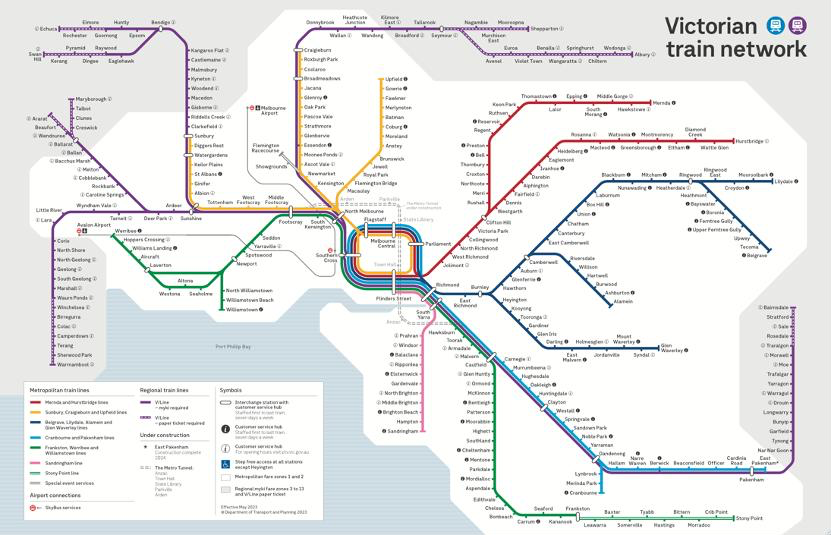
(data source: https://www.ptv.vic.gov.au/more/maps/#networkmaps)
Within this setting, the Cranbourne Line—the corridor analyzed in this study—runs roughly 50 km southeast from the CBD, threading through mature residential neighborhoods with a notable Chinese immigrant population. It is among the city’s highest-demand commuter corridors, carrying approximately 160,000 passengers per day and connecting major destinations such as Chadstone (Australia’s largest shopping centre), Monash University (Caulfield and Clayton), affluent precincts including Toorak and South Yarra, and the Dandenong Ranges. Given its role for the roughly 860,060 residents of Southeast Melbourne and its salience for transport and land-use decision-making, the empirical lens centers on dwellings located within 3 km of the line, where proximity effects are most credibly observed.
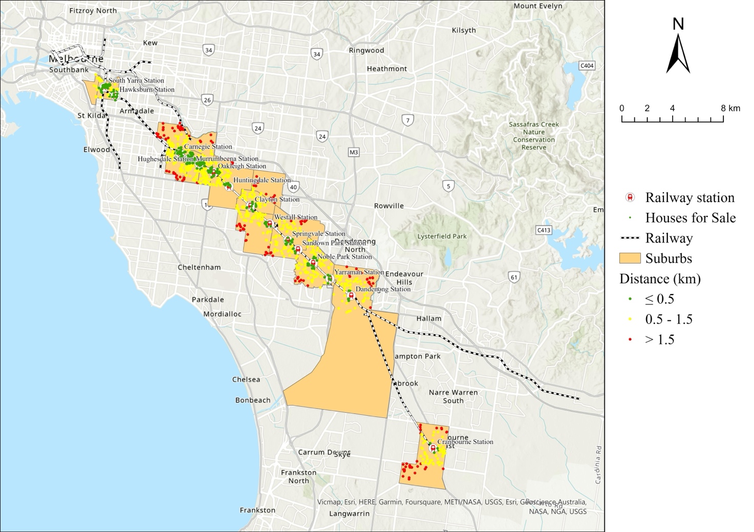
Figure 2. Cranbourne line and properties site map
(data source: original)
Observations regarding variables and measurement. Accessibility is measured by the distance from each property to the nearest rail station and the Central Business District (CBD). The accessibility of local amenities is quantified by the number of bus stations, schools, and hospitals within a 5-km radius. Residential attributes encompass the number of bedrooms, baths, available on-site parking, and the property's age. Neighborhood controls include median age, median weekly income, and labor-force participation, all assessed at the SA1 level. This configuration aims to separate the capitalization of rail access while appropriately accounting for structural features and socio-economic context.
3.3. Data analysis
3.3.1. Descriptive statistics and correlations
Table 1 defines the outcome and covariate blocks used in both the global OLS and the GWR: the dependent variable is unit residential price (AUD/m²); transportation accessibility is measured as distance to the nearest bus stop (disbustp), the nearest train station (distrain), and the CBD (discbd); local life-convenience is captured by counts of bus stops, hospitals, and schools within 5 km (numbustp, numhospital, numschool); residential property features include bedrooms, bathrooms, and age (numbed, numbath, age); and community demography comprises median age, median weekly income, and labor-force participation (median age, median income, labor).
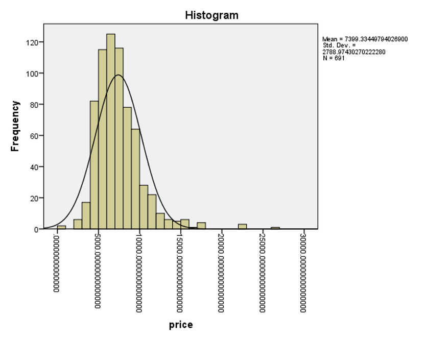
Descriptive statistics in Table 2 and the histogram in Figure 3 show a mean unit price of 7,399.33 AUD/m² with a standard deviation of 2,788.97 and a wide range from 5.94 to 26,969.7 AUD/m², indicating substantial dispersion across locations. This spread is consistent with heterogeneous accessibility and amenity conditions along the corridor; properties with stronger transport access generally transact at higher prices, whereas more peripheral or less connected locations trade at discounts. The price distribution is broadly compatible with an approximately normal shape.
The correlation matrix in Table 3 indicates that structural attributes co-vary positively with price: more bedrooms, bathrooms, and on-site parking are associated with higher unit values. Distance-based measures correlate negatively with price, consistent with an accessibility premium: coefficients for distance to the CBD, nearest station, and nearest bus stop are −0.592, −0.2917, and −0.2815, respectively. Service densities within 5 km correlate positively with price, with coefficients of 0.6156 for bus stops, 0.5705 for hospitals, and 0.4807 for schools. Overall, the signs and magnitudes align with the hedonic framework and motivate the multivariate models that follow .
|
Type |
Feature |
Name |
Data description |
|
Dependent Variable |
price |
Unit residential property land price per square meter |
|
|
Independent Variable |
Transportation accessibility |
disbustp distrain discbd |
Distance to the nearest bus stop |
|
Distance to the nearest train station |
|||
|
Distance to CBD |
|||
|
Life convenience |
numbustp |
Number of bus stops (5km) |
|
|
numhospital |
Number of hospitals (5km) |
||
|
numschool |
Number of Schools (5km) |
||
|
Residential property feature |
numbed |
Number of Bedroom |
|
|
numbath |
Number of Bathroom |
||
|
age |
Age of Built |
||
|
Community demography |
medianage |
Median Age |
|
|
medianincome |
Median Income (Weekly) |
||
|
labor |
Percentage of labour force |
The correlation matrix shows positive associations between price and structural attributes (bedrooms, bathrooms, and parking spaces), while price correlates negatively with distance-based accessibility measures. In particular, price is negatively correlated with distance to the CBD (discbd = −0.592) and with distances to stations and bus stops, and positively correlated with the density of bus stops (numbustp = 0.6156), hospitals (numhospital = 0.5705), and schools (numschool = 0.4807) within 5 km. These signs are consistent with the hedonic framework adopted for the global specification.
3.3.2. Global hedonic model
The global hedonic specification takes unit sale price (AUD/m²) as the outcome and includes covariates for accessibility (distances to the nearest bus stop, the nearest rail station, and the CBD), local services (counts of bus stops, schools, and hospitals within 5 km), dwelling attributes (bedrooms, bathrooms, on-site parking, and age), and neighbourhood socio-demographics (median age, median income, and labour-force participation). Estimation is conducted on a complete-case sample of N = 374 observations, yielding F(13, 360) = 77.96, p = 0.000, with R² = 0.738 and adjusted R² = 0.728.
Estimated coefficients are directionally and economically sensible. Variables meeting p < 0.10 include bedrooms, parking spaces, distance to station, distance to the CBD, bus stops (5 km), schools (5 km), median income, and labour-force participation. Among these, bedrooms, parking spaces, distance to the CBD, bus stops (5 km), and median income are significant at the 1% level; distance to station and labour-force participation at 5%; and schools (5 km) at 10%. Signs accord with expectation: additional bedrooms and on-site parking are associated with higher unit prices; greater separation from the CBD and from the nearest station is associated with lower unit prices; and denser provision of nearby bus stops and schools is associated with higher unit prices. Full coefficient tables and diagnostics appear in Table 4.
3.3.3. Geographically Weighted Regression (GWR)
To probe spatial non-stationarity, this paper estimate GWR for covariates exhibiting marked geographic variation. Results show that the station-access effect is not uniform across the corridor. The coefficient on distance to station spans [−718.9209, 420.3894] with a standard deviation of 174.6705, indicating pronounced heterogeneity in how proximity to rail is capitalized into prices along the Cranbourne Line. Cartographic outputs of local coefficients and related statistics are reported in the main results and the appendix.
Summary. In combination, the descriptive evidence, the global estimates, and the local (GWR) surfaces indicate that rail and CBD accessibility, local service densities, and core structural features are systematically related to per-m² prices, with substantive spatial variation in the accessibility–price gradient along the study corridor.
4. Empirical results and spatial diagnostics
4.1. Descriptive statistics analysis
|
Variable |
Mean |
Std. Dev. |
Min |
Max |
|
price |
7399.33 |
2788.97 |
5.94 |
26969.7 |
|
numbed |
2.72 |
1.19 |
0 |
10 |
|
numbath |
1.57 |
0.81 |
0 |
7 |
|
numparking |
1.44 |
0.80 |
0 |
6 |
|
age |
38.98 |
28.68 |
1 |
174 |
|
disbustop |
0.63 |
0.54 |
0.01 |
6.12 |
|
distrain |
1.47 |
1.94 |
0.05 |
23.97 |
|
discbd |
20.93 |
10.89 |
2.14 |
48.04 |
|
numbustp |
199.82 |
122.67 |
4 |
560 |
|
numhospital |
7.95 |
5.16 |
0 |
39 |
|
numschool |
56.13 |
27.35 |
2 |
199 |
|
medianage |
35.70 |
4.75 |
19 |
54 |
|
medianincome |
803.70 |
328.92 |
69 |
1743 |
|
labor |
0.55 |
0.11 |
0.11 |
0.89 |
(data source: original)
The analysis begins with descriptive statistics for all variables—minimum, maximum, mean, and standard deviation—reported in Table 2, with a histogram of the unit price displayed in Figure 2. The mean unit residential price is 7,399.33 AUD/m², accompanied by a sizable standard deviation of 2,788.97, indicating substantial dispersion in transaction values. This variability is further reflected in the wide range of observed prices, from 5.94 to 26,969.7 AUD/m². Such dispersion is consistent with uneven spatial conditions across the corridor: properties in locations with stronger transport accessibility typically transact at higher prices, whereas those in more peripheral or less accessible areas command lower values. Overall, the magnitude of the standard deviation underscores marked heterogeneity in the price data. In addition, the distributional pattern in Figure 1 suggests that the price variable is broadly consistent with an approximately normal form.
4.2. Correlation analysis
|
price |
numbed |
numbath |
numparking |
age |
disbustop |
distrain |
|
|
price |
1 |
||||||
|
numbed |
0.4017 |
1 |
|||||
|
numbath |
0.3609 |
0.6629 |
1 |
||||
|
numparking |
0.3406 |
0.4516 |
0.3566 |
1 |
|||
|
age |
-0.1571 |
-0.1224 |
-0.3182 |
-0.0713 |
1 |
||
|
disbustop |
-0.2815 |
-0.0328 |
-0.0758 |
-0.0168 |
0.2099 |
1 |
|
|
distrain |
-0.2917 |
0.0199 |
-0.0581 |
0.0287 |
0.3215 |
0.5177 |
1 |
|
discbd |
-0.592 |
0.0606 |
-0.1148 |
-0.0034 |
0.1029 |
0.3379 |
0.2244 |
|
numbustp |
0.6156 |
0.0089 |
0.1066 |
0.042 |
-0.0984 |
-0.2595 |
-0.2965 |
|
numhospital |
0.5705 |
0.13 |
0.2168 |
0.2171 |
-0.1735 |
-0.3103 |
-0.2537 |
|
numschool |
0.4807 |
-0.0471 |
0.0744 |
0.0554 |
-0.0905 |
-0.332 |
-0.3376 |
|
medianage |
0.13 |
0.1248 |
0.0291 |
0.1007 |
0.1216 |
0.0981 |
0.0261 |
|
medianincome |
0.5943 |
0.086 |
0.2105 |
0.1106 |
-0.1424 |
-0.2649 |
-0.3228 |
|
labor |
0.4217 |
-0.0831 |
0.1167 |
-0.0053 |
-0.2473 |
-0.2946 |
-0.3985 |
|
discbd |
numbustp |
numhospital |
numschool |
medianage |
medianincome |
labor |
|
|
price |
|||||||
|
numbed |
|||||||
|
numbath |
|||||||
|
numparking |
|||||||
|
age |
|||||||
|
disbustop |
|||||||
|
distrain |
|||||||
|
discbd |
1 |
||||||
|
numbustp |
-0.7173 |
1 |
|||||
|
numhospital |
-0.6545 |
0.6303 |
1 |
||||
|
numschool |
-0.6015 |
0.5238 |
0.557 |
1 |
|||
|
medianage |
-0.0285 |
-0.0268 |
-0.1035 |
0.0174 |
1 |
||
|
medianincome |
-0.5792 |
0.5702 |
0.5458 |
0.574 |
0.0093 |
1 |
|
|
labor |
-0.673 |
0.6029 |
0.5163 |
0.4737 |
-0.2667 |
0.595 |
1 |
Table 3 reports the pairwise correlation matrix across variables. For dwelling attributes, the number of bedrooms and bathrooms exhibits a positive association with unit price; that is, properties with more bedrooms or bathrooms tend to transact at higher values. By contrast, the distance-based accessibility measures are negatively correlated with price: the coefficients for distance to the nearest bus stop, rail station, and the CBD are −0.2815, −0.2917, and −0.592, respectively. Interpreted inversely, better accessibility (shorter distance) is associated with higher prices. Regarding local services, the correlations between price and the counts within 5 km of bus stops, hospitals, and schools are 0.6156, 0.5705, and 0.4807, respectively, indicating that denser service provision co-varies positively with unit prices.
4.3. Estimation and analysis of the hedonic price model
In this section, the outcome variable is the per-square-metre transaction price for 691 residential properties located along the rail corridor. The specification includes 13 covariates covering four domains: transportation accessibility, everyday service availability (living convenience), dwelling characteristics, and neighborhood socio-demographics. An ordinary least squares (OLS) hedonic model is employed to recover corridor-wide associations between these factors and unit prices. The objective is to quantify both the direction and magnitude of each relationship, thereby clarifying which attributes are most closely linked to price differentials. Interpretation emphasizes not only statistical significance but also economic significance (effect sizes and practical relevance), ensuring that the findings speak to both inferential validity and policy usefulness.
|
price |
Coef. |
Std. Err. |
t |
P>t |
|
numbed |
993.201 |
102.513 |
9.69 |
0.000 |
|
numbath |
-33.984 |
154.712 |
-0.22 |
0.826 |
|
numparking |
458.980 |
120.699 |
3.8 |
0.000 |
|
age |
-2.048 |
3.591 |
-0.57 |
0.569 |
|
disbustop |
-229.313 |
238.745 |
-0.96 |
0.337 |
|
distrain |
-139.868 |
56.781 |
-2.46 |
0.014 |
|
discbd |
-85.066 |
15.166 |
-5.61 |
0.000 |
|
numbustp |
6.290 |
1.054 |
5.97 |
0.000 |
|
numhospital |
18.535 |
24.754 |
0.75 |
0.454 |
|
numschool |
8.267 |
4.282 |
1.93 |
0.054 |
|
medianage |
23.657 |
20.370 |
1.16 |
0.246 |
|
medianincome |
2.133 |
0.378 |
5.64 |
0.000 |
|
labor |
-2713.769 |
1362.894 |
-1.99 |
0.047 |
|
_cons |
3494.817 |
1437.011 |
2.43 |
0.016 |
|
N |
374 |
|||
|
F(13, 360) |
77.96 |
|||
|
Prob > F |
0.000 |
|||
|
R-squared |
0.738 |
|||
|
Adj R-squared |
0.728 |
|||
|
Root MSE |
1666.9 |
|||
The statistical evaluation focuses on overall fit and the explanatory contribution of the regressors as inferred from the least-squares estimates. The dependent variable is the unit transaction price of residential property (AUD/m²). Estimation results are reported in Table 4.
The hedonic specification attains an R² of 0.748 and an adjusted R² of 0.728, indicating that the model explains 72.8% of the cross-sectional variation in unit prices. The joint significance test yields F(13, 360) = 77.96 with p = 0.00, confirming significance at the 1% level and supporting the model’s strong explanatory validity. In addition, most covariates are significant at 5% or better, suggesting that the chosen characteristics meaningfully account for price differences and that the fitted equation provides an adequate representation of the data.
At the variable level, numbed, numparking, distrain, discbd, numbustp, numschool, medianincome, and labor exhibit p-values < 0.10. Within this set, numbed, numparking, discbd, numbustp, and medianincome are significant at 1%; distrain and labor at 5%; and numschool at 10%. Signs are economically coherent: more bedrooms and on-site parking are associated with higher unit values, while greater distances to the nearest station and to the CBD are associated with lower values; denser local services (bus stops and schools within 5 km) co-vary positively with prices.
Turning to magnitudes, the estimated coefficient on numbed is 993.201 (statistically significant), implying that, holding other factors constant, each additional bedroom is associated with an increase of approximately AUD 993.201 per m². The coefficient on numparking is 458.980 (statistically significant), indicating that one additional parking space corresponds to roughly AUD 458.98 per m² higher unit price, ceteris paribus. Together, these results underscore the sizeable and positive contributions of core structural attributes—bedrooms and parking—to residential unit values along the corridor.
Regarding transportation access, the estimated coefficient on distance to the nearest station (distrain) is −139.868 and statistically significant, indicating a clear inverse gradient: for each additional kilometre from a station, the unit sale price falls by roughly AUD 139.87. This conforms to the a priori expectation that rail proximity is capitalized into value. A similar pattern holds for distance to the CBD (discbd), whose coefficient is −85.066 and significant; moving one kilometre farther from the metropolitan core is associated with a decrease of about AUD 85 per square metre, ceteris paribus.
Turning to local convenience, the coefficient on bus-stop density within 5 km (numstop) equals 6.290 and is significant, implying that each additional nearby bus stop is associated with an increase of approximately AUD 6.29 per square metre. The school count within 5 km (numschool) also enters positively and significantly at 8.267, suggesting that increments in proximate educational facilities are reflected in higher unit prices (≈ AUD 8.27 per additional school), holding other factors constant.
For neighbourhood conditions, median income (medianincome) carries a positive, significant coefficient of 2.133. Interpreted in levels, a one dollar increase in local median income corresponds to an estimated AUD 2.133 rise in unit price, all else equal. This aligns with the notion that stronger socio-economic profiles support higher willingness to pay.
Within the OLS hedonic framework, these results jointly indicate that structural attributes dominate on average: additional bedrooms and on-site parking exhibit the largest positive associations with per-m² prices, followed by access variables (distance to station and to the CBD). Among amenities, counts of nearby schools and hospitals within the specified catchment exert meaningful positive effects, reinforcing the role of everyday service availability in shaping market valuations along the corridor.
That said, the price-characteristics model estimated by ordinary least squares is a global specification. By construction, it imposes a single parameter for each covariate across all station areas, which can mask spatial non-stationarity and leave residual spatial autocorrelation unaddressed. Consequently, purely global estimates may understate or miss location-specific patterns in capitalization. To overcome these limitations, the subsequent analysis turns to geographically weighted regression (GWR), which relaxes the constant-parameter assumption and yields location-specific coefficients. This local modelling approach improves interpretive precision and overall fit, and it is better suited to diagnosing spatial heterogeneity in the determinants of residential unit prices along the Cranbourne corridor.
4.4. Estimation and analysis of the geographically weighted regression
Spatial relationships are unlikely to be constant across the corridor; the effect of a given attribute on unit prices can shift with location. Because the observations are distributed unevenly along the rail alignment, the magnitude—and occasionally the sign—of attribute–price associations may differ from one station catchment to another. To probe this spatial heterogeneity beyond the global hedonic benchmark, this paper estimates a Geographically Weighted Regression (GWR) in which the dependent variable remains the per-square-metre dwelling price for properties along the Cranbourne Line. GWR produces a set of location-specific coefficients for the same covariate blocks used in the OLS model (accessibility, local services, structure, and neighborhood context), enabling direct comparison between global averages and local responses. The resulting coefficient surfaces and associated diagnostics allow us to identify where capitalization of rail access and service bundles is strongest, where it weakens, and how these patterns align with the spatial structure of the corridor.
4.4.1. Kernel and bandwidth specification
GWR is a local regression technique: observations nearer to a target location receive greater weight than those farther away. This is implemented through a kernel (weight) function and a bandwidth parameter that together govern the size and influence of the local neighborhood. Given the linear, corridor-like distribution of the data and the varying point density around different stations, this research employs an adaptive kernel weighting scheme so that each local regression uses a comparable number of neighbors regardless of local sampling density. The bandwidth—i.e., the extent of the local neighborhood—is selected through an information-criterion/cross-validation procedure to balance bias and variance, thereby improving fit and the stability of local estimates. This specification is designed to yield robust location-specific parameters and to reflect genuine regional variation rather than noise arising from irregular observation spacing.
4.4.2. Geographical variability test
|
Variable |
F |
DOF |
F test |
DIFF of Criterion |
|
Intercept |
28.084 |
4.08 |
609.72 |
-108.542 |
|
numbed |
7.525 |
5.053 |
609.72 |
-28.861 |
|
numbath |
3.370 |
5.186 |
609.72 |
-6.251 |
|
numparking |
1.246 |
5.401 |
609.72 |
6.239 |
|
age |
1.958 |
4.669 |
609.72 |
1.682 |
|
disbustop |
1.710 |
4.699 |
609.72 |
2.995 |
|
distrain |
6.921 |
3.880 |
609.72 |
-19.825 |
|
discbd |
0.474 |
4.132 |
609.72 |
8.381 |
|
numbustp |
4.851 |
4.539 |
609.72 |
-12.884 |
|
numhospital |
4.068 |
3.827 |
609.72 |
-7.602 |
|
numschool |
1.355 |
3.669 |
609.72 |
3.804 |
|
medianage |
1.390 |
4.458 |
609.72 |
4.438 |
|
medianincome |
4.209 |
4.966 |
609.72 |
-10.572 |
|
labor |
0.996 |
4.761 |
609.72 |
6.844 |
During GWR specification, this research first screened covariates for spatial non-stationarity. To do so, this research estimated a global baseline that augments the hedonic controls with each dwelling’s longitude and latitude and then applied variability tests to the resulting global coefficients. Table 5 reports the outcomes of these diagnostics. Under the selection metric, a positive value of the “diff-Criterion” indicates no evidence of spatial variation in the corresponding parameter, whereas non-positive values point to geographically varying effects. On this basis, the following variables exhibit significant spatial variability: numbed (bedrooms), numbath (bathrooms), distrain (distance to the nearest rail station), numbustp (bus-stop count within the buffer), numhospital (hospital count), and medianincome (neighbourhood income). By contrast, numparking (on-site parking spaces), age (dwelling age), disbustp (distance to the nearest bus stop), discbd (distance to the CBD), numschool (school count), medianage (neighbourhood median age), and labor (labour-force participation) show no detectable spatial variability according to the same criterion. Consequently, the GWR is estimated using only the subset of covariates flagged as spatially varying—numbed, numbath, distrain, numbustp, numhospital, and medianincome—with the per-square-metre residential price as the dependent variable. This strategy ensures that local modelling effort is concentrated where parameters genuinely differ across space, while variables that behave globally are retained in their pooled (non-local) form.
4.4.3. Regression result
|
Variable |
Estimate |
Standard Error |
t(Est/SE) |
|
Intercept |
1569.7989 |
276.8873 |
5.6695 |
|
numbed |
874.4881 |
80.2898 |
10.8916 |
|
numbath |
82.3344 |
121.2878 |
0.6788 |
|
distrain |
-12.1714 |
8.2071 |
-1.4830 |
|
numbustp |
9.3065 |
0.9283 |
10.0254 |
|
numhospital |
56.8417 |
2.9904 |
19.0082 |
|
medianincome |
1.6684 |
0.3339 |
4.9972 |
Table 6 reports the GWR estimates for the subset of covariates identified as spatially varying. Except for numbath, whose local effect is not statistically distinguishable from zero, all other coefficients are significant. The local estimate for numbed is 874.4881, indicating a strong positive association between additional bedrooms and unit price, consistent with the global OLS benchmark. The coefficient on distrains equals −12.1714, confirming that greater separation from the nearest rail station is linked to lower per-m² values. Among convenience and neighborhood factors, the bus-stop count within 5 km (numbustp) carries a positive and significant coefficient of 9.3065, the hospital count (numhospital) enters at 56.8417, and median income (medianincome) at 1.6684; each point to higher unit prices where service density and socio-economic status are stronger. Overall, the direction and significance of the GWR coefficients closely mirror the OLS results, reinforcing the robustness of the baseline relationships while allowing for geographically varying intensities across the corridor.
|
Variable |
Mean |
Median |
STD |
Min |
Max |
Range |
|
Intercept |
1918.2795 |
2058.2628 |
1814.3240 |
-2777.0177 |
5764.6795 |
8541.6972 |
|
numbed |
677.0088 |
612.9522 |
440.3635 |
-181.7133 |
1698.8405 |
1880.5538 |
|
numbath |
-119.8000 |
-239.7589 |
426.9448 |
-1522.6875 |
742.8014 |
2265.4889 |
|
distrain |
-38.8792 |
-7.9860 |
174.6705 |
-718.9209 |
420.3894 |
1139.3103 |
|
numbustp |
9.0236 |
9.1421 |
5.0306 |
-0.6900 |
22.3151 |
23.0051 |
|
numhospital |
69.9837 |
61.5609 |
41.2920 |
-4.1845 |
189.7227 |
193.9072 |
|
medianincome |
2.4129 |
2.1227 |
1.7585 |
-0.8821 |
8.2329 |
9.1151 |
The GWR estimation yields location-specific parameters for each explanatory variable, enabling us to observe how effects differ across individual observations. To synthesize these local estimates, this research compute descriptive statistics for each coefficient; the summary is reported in Table 7, which lists the mean, median, standard deviation, minimum, maximum, and the dispersion range (max–min). The results show substantial variation both across variables and within any given variable, confirming spatial non-stationarity in the determinants of unit prices. In other words, the same attribute does not exert a uniform influence throughout the corridor; its magnitude and, in some cases, direction depend on spatial context. Consistent with this heterogeneity, the GWR specification delivers superior goodness-of-fit relative to the global linear model, indicating higher explanatory accuracy and more reliable local inference.
Interpreting the medians of the local coefficients is informative because they summarize the central tendency of the effects across more than half of the sample locations. In line with prior evidence, intrinsic dwelling characteristics remain the most potent contributors to price formation. Focusing on the spatially modelled blocks—transport accessibility, amenities, and community characteristics—Table 7 indicates that, within amenities, the hospital count (numhospital) exhibits the largest median absolute effect, followed by the bus-stop count (numbustp). The median coefficient on distance to the nearest rail station (distrain) ranks third and carries a negative sign, implying that greater separation from a station is associated with lower unit prices. Median neighbourhood income (medianincome) ranks fourth and is positive, consistent with higher local purchasing power supporting higher values. Taken together, the signs and relative magnitudes conform to expectations: accessibility penalties are negative, while richer service bundles and stronger socio-economic context are positively associated with residential unit prices, with the intensity of these associations varying meaningfully across space.
The standard deviation of the local regression coefficients quantifies dispersion around each variable’s mean effect and, by extension, the extent of spatial non-stationarity in how that variable relates to unit prices. Larger dispersion indicates greater place-to-place variability in influence. As reported in Table 7, the standard deviation for distance to the nearest station is 174.6705, signalling substantial regional differences in the valuation of rail proximity; among all predictors, this variable exhibits the most pronounced spatial variability, implying that the price sensitivity to access is far from uniform along the corridor. By comparison, the standard deviation for the hospital count is 41.2920, indicating meaningful but more moderate heterogeneity that likely reflects differing local preferences for healthcare access. In contrast, the income coefficient’s standard deviation of 1.7585 suggests relatively limited spatial variation in the income–price association.
Extrema of the local coefficients further delineate how effects vary across locations. For the station-distance variable, the minimum local coefficient is −718.9209 and the maximum is 420.3894. Thus, in some catchments an additional kilometre from the nearest station is associated with a decrease in unit price of up to 718.9209, whereas in other areas the same increase in distance corresponds to an increase in unit price of up to 420.3894. These opposing tails underscore the corridor’s strong spatial heterogeneity: depending on local conditions—such as noise exposure, crowding, walkability, parking supply, or the availability of alternative modes—greater separation from a station can either penalize or, in select contexts, be associated with higher residential values.
5. Discussion
On a per‑square‑metre basis, residential values increase with core structural attributes—most notably bedrooms and on‑site parking—and with the density of proximate services such as bus stops and schools within the local catchment. By contrast, distance penalties are evident for both the nearest rail station and the CBD, indicating that effective access to the trunk network and major employment is priced in. For a cross‑section, the global model exhibits strong fit and concentrates statistical significance on variables with direct behavioural channels (internal space, access/egress cost and convenience, everyday services). However, the local modelling layer makes it equally clear that these averages mask substantial geographic variation: the station‑distance gradient is materially steeper in some catchments than others, and in a few locations the relationship weakens or even reverses—an empirical signal that proximity benefits are being offset by local disamenities such as noise, air‑quality burdens, or crowding [20]. That pattern is also consistent with well‑known issues in hedonic prediction and segmentation, where attribute effects differ across submarkets and model performance improves when such heterogeneity is acknowledged [21].
Positioning these results against prior research shows both consistencies and useful divergences. Classic urban development perspectives underline that network investments reshape urban structure and land bids over time . Environmental‑quality studies demonstrate that households capitalize cleaner air and related amenities into housing prices, reinforcing why local externalities can attenuate transport premia when left unmitigated [22]. Amenity‑specific evidence further indicates that micro‑environmental benefits such as wider views and streetscape quality are reflected in transaction values and that urban ecological assets can raise willingness to pay in dense districts [23]. Broader policy frameworks around compact growth also mediate outcomes by aligning transport supply with place‑based development while heterogeneous landscape change and urbanization trajectories condition how accessibility interacts with built form [24]. Consistent with the present findings, corridor and station‑area studies in transit‑oriented settings detect price premia linked to rail access and station‑area design, and network‑scale work on rail accessibility likewise reports positive associations with residential values when measured with realistic access metrics. At the same time, local‑model evidence shows that allowing coefficients to vary across space improves fit and recovers structure missed by global specifications, with spatial heterogeneity in price formation repeatedly observed across multi‑center urban regions. Temporal dynamics also matter around new or upgraded lines; prices may react around opening and early operations in ways that are not captured by static averages [25]. Comparable applications in other contexts confirm that geographically weighted approaches can reveal corridors and neighborhoods where accessibility premia are strongest or weakest [26]. A parallel strand on environmental externalities—such as pollution exposure—corroborates the mechanism by which local disamenities can dampen proximity benefits [27]. General syntheses of transit’s economic impacts point to these same channels of accessibility and amenity working in tandem [28]. Finally, consistent with the positive amenity coefficients, school‑quality meta‑reviews and housing studies document strong capitalization of educational services [29], and building‑quality research similarly links construction attributes to higher valuations [30].
Translating these patterns into action, corridor planning should priorities interventions where local coefficients indicate stronger accessibility capitalization rather than spreading resources uniformly along the line. In middle‑ring segments with steep station‑distance gradients, priorities TOD up‑zoning and mixed‑use infill, remove micro‑barriers to walk access (block permeability, mid‑block crossings, continuous footpaths), and tighten feeder‑bus headways to clock‑face schedules that reliably meet trunk services; safe, direct cycling links to station entries should be delivered as part of the same access package . Where gradients are flat or locally reversed, treat the causes: mitigate disamenities through rail‑noise abatement and platform crowding management; redesign station forecourts to reduce conflict between buses, kiss‑and‑ride, and pedestrians; and re‑stitch stations to adjacent retail or civic anchors so that proximity translates into realized utility [31]. These implementation choices align with value‑capture theory and betterment considerations, suggesting room for calibrated developer contributions and density bonuses where capitalization is demonstrably strong . Distribution‑sensitive evidence on transit premia also cautions that benefits are not uniform across the price spectrum, arguing for station‑area policies that tailor inclusionary housing and affordability instruments to local market segments [32]. Corridor case studies further show that granular, line‑specific hedonic work can guide planning where rail access and urban design interact most strongly and that even in historic polycentric settings, improving secondary centers’ accessibility can reshape local land‑value patterns.
6. Conclusion
This study investigated how urban rail accessibility capitalizes into residential unit prices along Melbourne’s Cranbourne Line, against the backdrop of sustained investment in transit‑oriented development and the policy imperative to understand place‑specific accessibility premia. A dwelling‑level dataset was assembled by geocoding transactions and merging structural attributes with SA1 socio‑demographics and a curated inventory of local amenities and transport indicators; a two‑stage empirical strategy then disentangled corridor‑wide regularities from spatially heterogeneous effects. In the first stage, a transparent hedonic price model related unit prices (AUD/m²) to distances to the nearest rail station and to the CBD, to the density of proximate services (bus stops, schools, hospitals), and to core structural and neighborhood characteristics; in the second stage, geographically weighted regression allowed key coefficients to vary over space, reflecting the plausible non‑stationarity of capitalization along a multi‑station corridor. The results are economically coherent: dwellings closer to stations and to the CBD are associated with higher unit prices; denser bundles of local amenities correlate with higher prices; and structural attributes such as bedrooms and on‑site parking carry positive associations. At the same time, the local modelling shows that these relationships are not uniform: the distance‑to‑station gradient is stronger in certain catchments than others, pointing to segments where accessibility constraints bind more tightly and where planning interventions are likely to yield larger returns. These conclusions are consistent with broader syntheses on transit’s economic effects and with evidence that both accessibility and local amenities are priced in by households.
From a critical perspective, the paper’s primary contributions lie in the integration of micro‑level transactions with fine‑grained neighborhood and accessibility measures, in a design that supports both corridor‑wide inference and explicitly mapped local heterogeneity. This dual‑scale evidence is directly usable for station‑area planning, TOD up‑zoning, and last‑mile service design because it indicates not only that accessibility and amenities matter on average, but also where and by how much they matter along the line. Limitations remain and motivate future work. First, causal identification is constrained by potential placement endogeneity; a next step is to embed quasi‑experimental designs around exogenous timing (e.g., level‑crossing removals, station rebuilds) or to leverage instruments tied to historical alignments and engineering constraints. Second, the present analysis is cross‑sectional; panel data with repeated sales or multi‑year transaction windows would permit fixed effects and capture temporal adjustment. Third, Euclidean distance is a coarse proxy for generalised travel cost; integrating realistic network travel times, service headways, and reliability would align measures with commuter utility. Fourth, omitted local disamenities and amenities—rail noise, air quality, school‑quality indices, crime risk, and access to green space—should be layered into the model, drawing on environmental‑valuation and school‑quality literatures to calibrate effect sizes. Fifth, distribution‑aware estimators and robustness checks (quantile/robust regression, spatial error diagnostics) should complement the OLS baseline and GWR surfaces in future extensions. Finally, financing strategies should be calibrated to local capitalization patterns so that corridor improvements can be funded without exacerbating exclusion, using betterment and value‑capture overlays where appropriate.
References
[1]. Benjamin, J., & Sirmans, G. S. (1996). Mass transportation, apartment rent and property values. Journal of Real Estate Research, 12(1), 1–8.
[2]. Cervero, R., & Duncan, M. (2002). Land value impacts of rail transit services in Los Angeles County. Report prepared for National Association of Realtors and Urban Land Institute.
[3]. Debrezion, G., Pels, E., & Rietveld, P. (2011). The impact of rail transport on real estate prices: an empirical analysis of the Dutch residential property market. Urban Studies, 48(5), 997–1015.
[4]. Brunsdon, C., Fotheringham, A. S., & Charlton, M. E. (1996). Geographically weighted regression: a method for exploring spatial nonstationarity. Geographical Analysis, 28(4), 281–298.
[5]. Bitter, C., Mulligan, G. F., & Dall’erba, S. (2007). Incorporating spatial variation in residential property attribute prices: A comparison of geographically weighted regression and the spatial expansion method. Journal of Geographical Systems, 9, 7–27.
[6]. Wen, H., Jin, Y., & Zhang, L. (2017). Spatial heterogeneity in implicit residential property prices: Evidence from Hangzhou, China. International Journal of Strategic Property Management, 21(1), 15–28.
[7]. Lu, B., Charlton, M., & Fotheringhama, A. S. (2011). Geographically weighted regression using a non-Euclidean distance metric with a study on London residential property price data. Procedia Environmental Sciences, 7, 92–97.
[8]. Ren, P., Li, Z., Cai, W., Ran, L., & Gan, L. (2021). Heterogeneity analysis of urban rail transit on residential property with different price levels: A case study of Chengdu, China. Land, 10(12), 1330.
[9]. Mathur, S. (2020). Impact of transit stations on residential property prices across entire price spectrum: A quantile regression approach. Land Use Policy, 99, 104828.
[10]. Suhaimi, N. A., Maimun, N. H. A., & Sa'at, N. F. (2021). Does rail transport impact residential property prices and rents? Planning Malaysia, 19, .
[11]. Chorus, P., & Bertolini, L. (2011). An application of the node place model to explore the spatial development dynamics of station areas in Tokyo. Journal of Transport and Land Use, 4(1), 45–58.
[12]. Knaap, G. J., Ding, C., & Hopkins, L. D. (2001). Do plans matter? The effects of light rail plans on land values in station areas. Journal of Planning Education and Research, 21(1), 32–39.
[13]. Haque, M. M., Chin, H. C., & Debnath, A. K. (2013). Sustainable, safe, smart—three key elements of Singapore’s evolving transport policies. Transport Policy, 27, 20–31.
[14]. Sirmans, S., Macpherson, D., & Zietz, E. (2005). The composition of hedonic pricing models. Journal of Real Estate Literature, 13(1), 1–44.
[15]. Hill, R. J. (2013). Hedonic price indexes for residential property: A survey, evaluation and taxonomy. Journal of Economic Surveys, 27(5), 879–914.
[16]. Kang, C. D. (2019). Spatial access to metro transit villages and residential property prices in Seoul, Korea. Journal of Urban Planning and Development, 145(3), 05019010.
[17]. Duan, J., Tian, G., Yang, L., & Zhou, T. (2021). Addressing the macroeconomic and hedonic determinants of residential property prices in Beijing Metropolitan Area, China. Habitat International, 113, 102374.
[18]. Hall, P. (2014). Cities of tomorrow: An intellectual history of urban planning and design since 1880. John Wiley & Sons.
[19]. Clapp, J. M., & Giaccotto, C. (1998). Residential hedonic models: A rational expectations approach to age effects. Journal of Urban Economics, 44(3), 415–437.
[20]. Eshet, T., Ayalon, O., & Shechter, M. (2005). A critical review of economic valuation studies of externalities from incineration and landfilling. Waste Management & Research, 23(6), 487–504.
[21]. Goodman, A. C., & Thibodeau, T. G. (2003). Residential property market segmentation and hedonic prediction accuracy. Journal of Residential Property Economics, 12(3), 181–201.
[22]. Harrison Jr, D., & Rubinfeld, D. L. (1978). Hedonic residential property prices and the demand for clean air. Journal of Environmental Economics and Management, 5(1), 81–102.
[23]. Rosenzweig, C., Solecki, W. D., Blake, R., Bowman, M., Faris, C., Gornitz, V., & Zimmerman, R. (2011). Developing coastal adaptation to climate change in the New York City infrastructure-shed: Process, approach, tools, and strategies. Climatic Change, 106, 93–127.
[24]. Wang, Y., & Baddeley, M. (2016). The problem of land value betterment: A simplified agent-based test. The Annals of Regional Science, 57, 413–436.
[25]. McMillen, D. P., & McDonald, J. (2004). Reaction of residential property prices to a new rapid transit line: Chicago's Midway Line, 1983–1999. Real Estate Economics, 32(3), 463–486.
[26]. Munshi, T. (2020). Accessibility, infrastructure provision and residential land value: Modelling the relation using geographic weighted regression in the city of Rajkot, India. Sustainability, 12(20), 8615.
[27]. Nam, K. M., Ou, Y., Kim, E., & Zheng, S. (2022). Air pollution and residential property values in Korea: A hedonic analysis with long-range transboundary pollution as an instrument. Environmental and Resource Economics, 82(2), 383–407.
[28]. Neuwirth, R. (1990). Economic impacts of transit on cities. Transportation Research Record, 1274, 142–149.
[29]. Nguyen-Hoang, P., & Yinger, J. (2011). The capitalization of school quality into residential property values: A review. Journal of Residential Property Economics, 20(1), 30–48.
[30]. Ooi, J. T., Le, T. T., & Lee, N. J. (2014). The impact of construction quality on residential property prices. Journal of Residential Property Economics, 26, 126–138.
[31]. Ruo-Qi, L., & Jun-Hong, H. (2020, September). Prediction of residential property price along the urban rail transit line based on GA-BP model and accessibility. In 2020 IEEE 5th International Conference on Intelligent Transportation Engineering (ICITE) (pp. 487–492). IEEE.
[32]. Wang, Y., Feng, S., Deng, Z., & Cheng, S. (2016). Transit premium and rent segmentation: A spatial quantile hedonic analysis of Shanghai Metro. Transport Policy, 51, 61–69.
Cite this article
Pan,G. (2025). Rail Accessibility and Residential Unit Prices: Evidence from Melbourne’s Cranbourne Line. Advances in Economics, Management and Political Sciences,231,6-26.
Data availability
The datasets used and/or analyzed during the current study will be available from the authors upon reasonable request.
Disclaimer/Publisher's Note
The statements, opinions and data contained in all publications are solely those of the individual author(s) and contributor(s) and not of EWA Publishing and/or the editor(s). EWA Publishing and/or the editor(s) disclaim responsibility for any injury to people or property resulting from any ideas, methods, instructions or products referred to in the content.
About volume
Volume title: Proceedings of ICEMGD 2025 Symposium: Resilient Business Strategies in Global Markets
© 2024 by the author(s). Licensee EWA Publishing, Oxford, UK. This article is an open access article distributed under the terms and
conditions of the Creative Commons Attribution (CC BY) license. Authors who
publish this series agree to the following terms:
1. Authors retain copyright and grant the series right of first publication with the work simultaneously licensed under a Creative Commons
Attribution License that allows others to share the work with an acknowledgment of the work's authorship and initial publication in this
series.
2. Authors are able to enter into separate, additional contractual arrangements for the non-exclusive distribution of the series's published
version of the work (e.g., post it to an institutional repository or publish it in a book), with an acknowledgment of its initial
publication in this series.
3. Authors are permitted and encouraged to post their work online (e.g., in institutional repositories or on their website) prior to and
during the submission process, as it can lead to productive exchanges, as well as earlier and greater citation of published work (See
Open access policy for details).
References
[1]. Benjamin, J., & Sirmans, G. S. (1996). Mass transportation, apartment rent and property values. Journal of Real Estate Research, 12(1), 1–8.
[2]. Cervero, R., & Duncan, M. (2002). Land value impacts of rail transit services in Los Angeles County. Report prepared for National Association of Realtors and Urban Land Institute.
[3]. Debrezion, G., Pels, E., & Rietveld, P. (2011). The impact of rail transport on real estate prices: an empirical analysis of the Dutch residential property market. Urban Studies, 48(5), 997–1015.
[4]. Brunsdon, C., Fotheringham, A. S., & Charlton, M. E. (1996). Geographically weighted regression: a method for exploring spatial nonstationarity. Geographical Analysis, 28(4), 281–298.
[5]. Bitter, C., Mulligan, G. F., & Dall’erba, S. (2007). Incorporating spatial variation in residential property attribute prices: A comparison of geographically weighted regression and the spatial expansion method. Journal of Geographical Systems, 9, 7–27.
[6]. Wen, H., Jin, Y., & Zhang, L. (2017). Spatial heterogeneity in implicit residential property prices: Evidence from Hangzhou, China. International Journal of Strategic Property Management, 21(1), 15–28.
[7]. Lu, B., Charlton, M., & Fotheringhama, A. S. (2011). Geographically weighted regression using a non-Euclidean distance metric with a study on London residential property price data. Procedia Environmental Sciences, 7, 92–97.
[8]. Ren, P., Li, Z., Cai, W., Ran, L., & Gan, L. (2021). Heterogeneity analysis of urban rail transit on residential property with different price levels: A case study of Chengdu, China. Land, 10(12), 1330.
[9]. Mathur, S. (2020). Impact of transit stations on residential property prices across entire price spectrum: A quantile regression approach. Land Use Policy, 99, 104828.
[10]. Suhaimi, N. A., Maimun, N. H. A., & Sa'at, N. F. (2021). Does rail transport impact residential property prices and rents? Planning Malaysia, 19, .
[11]. Chorus, P., & Bertolini, L. (2011). An application of the node place model to explore the spatial development dynamics of station areas in Tokyo. Journal of Transport and Land Use, 4(1), 45–58.
[12]. Knaap, G. J., Ding, C., & Hopkins, L. D. (2001). Do plans matter? The effects of light rail plans on land values in station areas. Journal of Planning Education and Research, 21(1), 32–39.
[13]. Haque, M. M., Chin, H. C., & Debnath, A. K. (2013). Sustainable, safe, smart—three key elements of Singapore’s evolving transport policies. Transport Policy, 27, 20–31.
[14]. Sirmans, S., Macpherson, D., & Zietz, E. (2005). The composition of hedonic pricing models. Journal of Real Estate Literature, 13(1), 1–44.
[15]. Hill, R. J. (2013). Hedonic price indexes for residential property: A survey, evaluation and taxonomy. Journal of Economic Surveys, 27(5), 879–914.
[16]. Kang, C. D. (2019). Spatial access to metro transit villages and residential property prices in Seoul, Korea. Journal of Urban Planning and Development, 145(3), 05019010.
[17]. Duan, J., Tian, G., Yang, L., & Zhou, T. (2021). Addressing the macroeconomic and hedonic determinants of residential property prices in Beijing Metropolitan Area, China. Habitat International, 113, 102374.
[18]. Hall, P. (2014). Cities of tomorrow: An intellectual history of urban planning and design since 1880. John Wiley & Sons.
[19]. Clapp, J. M., & Giaccotto, C. (1998). Residential hedonic models: A rational expectations approach to age effects. Journal of Urban Economics, 44(3), 415–437.
[20]. Eshet, T., Ayalon, O., & Shechter, M. (2005). A critical review of economic valuation studies of externalities from incineration and landfilling. Waste Management & Research, 23(6), 487–504.
[21]. Goodman, A. C., & Thibodeau, T. G. (2003). Residential property market segmentation and hedonic prediction accuracy. Journal of Residential Property Economics, 12(3), 181–201.
[22]. Harrison Jr, D., & Rubinfeld, D. L. (1978). Hedonic residential property prices and the demand for clean air. Journal of Environmental Economics and Management, 5(1), 81–102.
[23]. Rosenzweig, C., Solecki, W. D., Blake, R., Bowman, M., Faris, C., Gornitz, V., & Zimmerman, R. (2011). Developing coastal adaptation to climate change in the New York City infrastructure-shed: Process, approach, tools, and strategies. Climatic Change, 106, 93–127.
[24]. Wang, Y., & Baddeley, M. (2016). The problem of land value betterment: A simplified agent-based test. The Annals of Regional Science, 57, 413–436.
[25]. McMillen, D. P., & McDonald, J. (2004). Reaction of residential property prices to a new rapid transit line: Chicago's Midway Line, 1983–1999. Real Estate Economics, 32(3), 463–486.
[26]. Munshi, T. (2020). Accessibility, infrastructure provision and residential land value: Modelling the relation using geographic weighted regression in the city of Rajkot, India. Sustainability, 12(20), 8615.
[27]. Nam, K. M., Ou, Y., Kim, E., & Zheng, S. (2022). Air pollution and residential property values in Korea: A hedonic analysis with long-range transboundary pollution as an instrument. Environmental and Resource Economics, 82(2), 383–407.
[28]. Neuwirth, R. (1990). Economic impacts of transit on cities. Transportation Research Record, 1274, 142–149.
[29]. Nguyen-Hoang, P., & Yinger, J. (2011). The capitalization of school quality into residential property values: A review. Journal of Residential Property Economics, 20(1), 30–48.
[30]. Ooi, J. T., Le, T. T., & Lee, N. J. (2014). The impact of construction quality on residential property prices. Journal of Residential Property Economics, 26, 126–138.
[31]. Ruo-Qi, L., & Jun-Hong, H. (2020, September). Prediction of residential property price along the urban rail transit line based on GA-BP model and accessibility. In 2020 IEEE 5th International Conference on Intelligent Transportation Engineering (ICITE) (pp. 487–492). IEEE.
[32]. Wang, Y., Feng, S., Deng, Z., & Cheng, S. (2016). Transit premium and rent segmentation: A spatial quantile hedonic analysis of Shanghai Metro. Transport Policy, 51, 61–69.