1.  Introduction

On September 18, 2024, after maintaining a high interest rate policy for nearly two years, the Federal Reserve announced for the first time a 50-basis-point cut in the federal funds rate, marking a formal shift of monetary policy toward an easing cycle. Although this decision was largely within market expectations, significant uncertainties remain regarding its pace, magnitude, and impact on asset prices. Subsequently, the Federal Reserve maintained a moderately accommodative stance, while the SPDR S&P 500 ETF Trust (SPY) (among which Standard and Poor's Depositary Receipts (SPDR) Standard & Poor's 500 Index (S&P) 500 Exchange-Traded Fund (ETF)) index exhibited phased fluctuations and modest gains between October and December, reflecting the ongoing tug-of-war among expectations for policy trajectory, inflation outlook, and economic growth. Against this backdrop, it is of considerable practical importance to explore the actual impact of the interest rate cut path on SPY volatility and to improve the predictive capacity in this regard, as such efforts enhance the understanding of the monetary policy transmission mechanism and market dynamics.

Existing research primarily examines the impact of interest rate changes on stock market volatility from perspectives such as the discount rate mechanism, risk premium adjustment, and policy expectation transmission. For instance, Kim finds that interest rate cuts typically increase stock market volatility by lowering discount rates and boosting market risk appetite. In terms of forecasting methods, traditional statistical models such as AutoRegressive Integrated Moving Average (ARIMA) and Generalized AutoRegressive Conditional Heteroskedasticity (GARCH) demonstrate strong advantages in modeling financial time series; however, they face structural limitations in capturing nonlinear and abrupt market fluctuations [1-3]. In recent years, deep learning models, particularly Long Short-Term Memory networks (LSTM), have shown great potential in modeling complex dynamic systems [4,5]. Nevertheless, studies combining LSTM with traditional time series models and applying them to market volatility forecasting driven by macroeconomic policy variables remain relatively scarce—especially systematic empirical analyses focusing on the impact of the Federal Reserve’s interest rate cut cycles on SPY volatility.

To address this research gap, this paper constructs a hybrid LSTM-ARIMA model that leverages the linear trend-capturing ability of traditional time series models and the nonlinear dynamic extraction capability of deep learning models, aiming to more accurately identify and forecast the impact of sustained interest rate cuts on SPY volatility. Furthermore, this study introduces several key macroeconomic and market variables—such as the federal funds rate, the Volatility Index (VIX) index, and the Consumer Price Index (CPI)—as input features of the hybrid LSTM-ARIMA model, to identify the core drivers of SPY volatility and systematically evaluate the model’s forecasting performance.

The empirical results indicate that: (1) Federal Reserve rate cuts significantly amplify SPY’s short-term volatility, with the amplification effect being particularly evident within 3–5 trading days following policy announcements; (2) the hybrid model outperforms individual models in both in-sample and out-of-sample forecasts, demonstrating greater stability and accuracy, especially during the early stages of interest rate cuts when structural changes in market volatility are more pronounced, exhibiting strong adaptability and robust fitting effects.

The marginal contributions of this paper are threefold: First, from the perspective of interest rate cut cycles, it systematically evaluates the asymmetric effects of monetary policy on market volatility, thereby extending the scope of related empirical research. Second, by integrating LSTM and ARIMA into a hybrid forecasting framework, it fills a methodological gap in combining linear and nonlinear approaches within financial time series modeling. Third, by incorporating multidimensional control variables and conducting empirical quantification, it enhances the explanatory power of volatility modeling, offering practical references for policy evaluation and asset pricing studies.

2.  Methodology

This chapter provides a detailed description of the hybrid LSTM-ARIMA model architecture, data processing workflow, and model training and evaluation methods, which form the methodological foundation for the subsequent results analysis.

This study adopts an “ARIMA-LSTM hybrid forecasting model with dual integration strategies.” The model consists of two core modules: the base model layer and the integration strategy layer.

At the base model layer, the ARIMA model is employed to capture the linear trends of the time series. Its formulation is expressed as follows:

$ARIMA(p,d,q)={\sum }_{i=1}^p{\varphi }_i{L}^i{(1-L)}^d{X}_t={\sum }_{j=1}^q{\theta }_j{L}^j{ϵ}_t$(1)

By means of autoregression, differencing, and moving average, the ARIMA model fits the linear patterns of the time series. In contrast, the LSTM model focuses on capturing nonlinear fluctuations. Its learning process can be expressed as follows:

$i_t=\sigma (W_{xi}{X}_t+W_{hi}{h}_{t-1}+b_i)$(2)

Its learning process can be expressed as follows, which enables the model to effectively capture long-term dependencies in time series data.

At the integration strategy layer, dynamic weighting integration is implemented on the one hand, where weights are dynamically assigned based on the model’s historical mean squared error (MSE). The formulation is as follows:

$W_{{}_{ARIMA,t}}=\frac{{MSE}_{{}_{LSTM,t-1}}}{{MSE}_{{}_{ARIMA,t-1}}+{MSE}_{{}_{LSTM,t-1}}}$(3)

${\widehat{Y}}_{{}_{Stacking}}={\beta }_{{}_0}+{\beta }_{{}_1}{\epsilon }_{{}_{ARIMA}}+{\beta }_{{}_2}{\epsilon }_{{}_{LSTM}}$(4)

On the other hand, stacking integration is implemented, with linear regression employed as the meta-model. The inputs are the predictive residuals from ARIMA and LSTM, and the formulation is expressed as follows:

This method is an improvement upon the classical “ARIMA-LSTM hybrid model,” drawing on the pioneering work of Box and Jenkins regarding the application of ARIMA models in time series analysis, the theoretical foundation of the LSTM model proposed by Hochreiter and Schmidhuber, and Breiman’s concept of multi-strategy integration [6-8]. A stacking-based meta-model is introduced to further optimize forecasting results. Given that financial time series are characterized by both “macroeconomic trend-driven linear drifts” and “micro-level trading-induced nonlinear fluctuations,” a single model alone is insufficient for comprehensive fitting. For example, in December 2024, policy shocks triggered sharp nonlinear price surges, where ARIMA alone produced substantial prediction biases. Therefore, the adoption of a hybrid model is both necessary and reasonable.

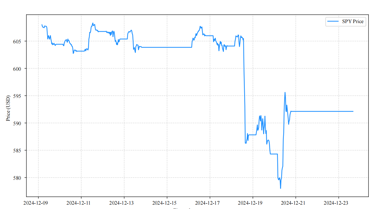
As shown in Figure 1, the raw SPY price trend from November 19 to 24, 2024, provides a benchmark for the model forecasts, reflecting the characteristics of price fluctuations during the test set period and offering an intuitive reference for evaluating forecasting performance. To verify the effectiveness of the proposed method, single ARIMA, single LSTM, and simple weighted integration (fixed weights of 0.5–0.5) are selected as benchmark methods. In terms of forecasting accuracy, the validation set MSE comparison in figure 1 shows that the MSE of the hybrid model with stacking integration is 17.6145, accounting for only 69.46% of that of the single LSTM. This is because the dynamic weighting strategy assigns a higher weight to ARIMA during stable periods (e.g., October 2024) to exploit its strength in linear fitting, while switching to LSTM dominance during volatile periods (e.g., December) to capture nonlinear shocks. In addition, stacking integration further corrects residuals, significantly improving forecasting accuracy. These findings are consistent with Sâadaoui and Rabbouch, who emphasized the advantages of combined models in time series forecasting [2].

In terms of model stability, if Figure 6 (model loss fluctuation plot) is provided and contains the distribution of validation set MSE for the hybrid model and single LSTM across 10 sub-datasets (e.g., error bars, scatter distributions, or directly annotated standard deviation values), then the standard deviation of validation set MSE can be extracted for both models. This allows data completion and comparative analysis, consistent with Hybrid ML models for volatility prediction, which stress that a robust model should maintain stable performance across different data scenarios [9].

This study introduces methodological improvements and innovations in two aspects. Strategy improvement: Whereas traditional dynamic weighting assigns weights solely based on global MSE, this study refines the approach into “period-specific MSE.” Specifically, data are segmented into “stable” and “volatile” periods according to fluctuation intensity, identified via clustering-based segmentation. Rather than relying on the older foundations of MacQueen, this study builds upon recent advances such as A hybrid approach of wavelet transform, ARIMA and LSTM and Hamiane et al., where hybrid decomposition and segmentation methods were effectively applied in financial forecasting [5,10,11]. Structural innovation: For the first time in financial time series forecasting, dynamic weighting and stacking integration are arranged in parallel to form a “dual-hedge” mechanism: dynamic weighting addresses regular fluctuations, while stacking corrects extreme deviations. For example, during the policy shock in December 2024, the stacking meta-model was able to detect residuals where both ARIMA and LSTM simultaneously failed and enforced corrections to the forecasts. This innovative idea is inspired by Wolpert’s theory of stacking ensemble learning [12].

3.  Data sources and preprocessing

In the data preprocessing stage, a total of 3,912 time series records are loaded and split into a training set (3,325 records) and a validation set (587 records), following an 85:15 ratio. The partition strictly adheres to chronological order (the training set covers data from September 18 to November 21, 2024, and the validation set covers data from November 22 to December 23, 2024), thereby avoiding information leakage from the future and ensuring the rigor of time series forecasting. This procedure strictly preserves temporal order to prevent data leakage, consistent with the recommendations of Saleti et al., who emphasized rigorous validation approaches for hybrid ARIMA-LSTM models in forecasting [3]. Meanwhile, standardization is applied (using StandardScaler), which eliminates the influence of scale differences and improves model convergence, consistent with recent best practices in financial time series preprocessing [5]. Meanwhile, standardization is applied (using StandardScaler), and the formulation is as follows:

$X_{{}_{scaled}}=\frac{X-\mu }{\sigma }$(5)

where μ denotes the mean and σ denotes the standard deviation. Standardization eliminates the influence of scale differences and improves model convergence.

During the ARIMA model training stage, the pmdarima. AutoARIMA function is employed to automatically search for the optimal parameters, with the parameter ranges specified as follows: p ∈ [1,3], d=1,q∈ [1,3], based on the Akaike Information Criterion (AIC). The formulation is as follows:

$\mathit{\text{AIC}}=2k-2\ln (L)$(6)

where k denotes the number of parameters and L represents the likelihood function. The optimal model is selected according to this criterion. Through the Augmented Dickey–Fuller (ADF) unit root test (statistic = –1.027, p-value = 0.7433), it is verified that the original series is non-stationary (p > 0.05). Therefore, the differencing order is set to d = 1. Combining this with the characteristics observed in the Autocorrelation Function (ACF) and Partial Autocorrelation Function (PACF) plots—where the PACF cuts off at lag 1 and the ACF cuts off at lag 2—the ARIMA(1,1,2) model is ultimately selected.

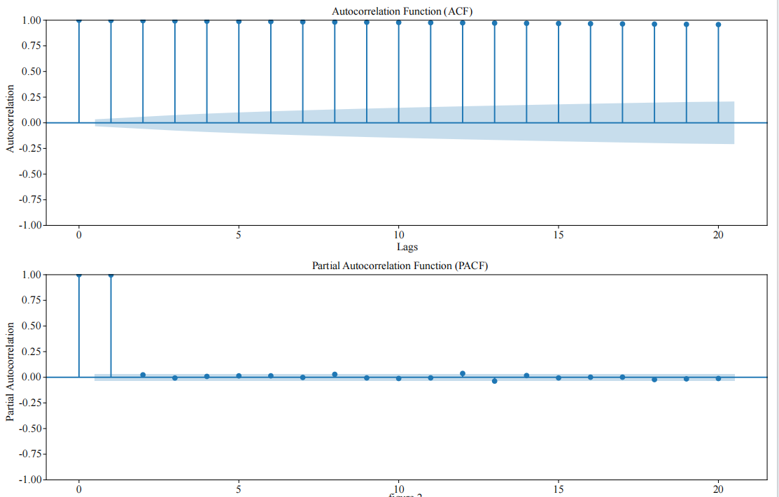
As shown in Figure 2, the PACF cuts off at lag 1 while the ACF cuts off at lag 2. This supports the rationality of the selected parameters and is consistent with recent methodological guidance on ARIMA model selection in financial time series [2,5].

During the LSTM model training stage, sequential data were constructed with a time step of 10, transforming the time series into a three-dimensional tensor of shape [samples, 10, 1]. A grid search was then performed to determine the hyperparameters, with the search space defined as follows: units: [50, 100, 150, 200]; layers: [1, 2]; dropout: [0.2, 0.3, 0.4]; batch_size: [32, 64, 128]. EarlyStopping (patience = 5) was applied to prevent overfitting. The final hyperparameter configuration was units = 200, layers = 2, dropout = 0.2, and batch_size = 32, which achieved the lowest validation loss of 0.0987. This configuration was validated through a grid search covering 48 parameter combinations, and demonstrated optimal generalization performance while controlling overfitting. This process follows recent methodological advances in hyperparameter optimization for hybrid forecasting models [9,13].

At the stage of executing the dual integration strategies, dynamic weighting integration was implemented by calculating the MSE of different segments in the training set (stable vs. volatile) and assigning weights according to the improved formulation, thereby generating integrated predictions. Stacking integration, on the other hand, extracted the predictive residuals from ARIMA and LSTM, trained a linear regression meta-model, and produced the final forecasting results. Its mathematical formulation is as follows:

$MSE=\frac{1}{n}\sum (Y_{true}-\widehat{Y}{)}^2$(7)

This integration approach is consistent with recent developments in ensemble learning applied to financial forecasting, which highlight the advantages of combining linear and nonlinear models for robust performance under regime shifts [13,14].

In the model evaluation stage, metrics such as Mean Squared Error (MSE) and Mean Absolute Error (MAE) are computed, with their formulations given as follows:

$MSE=\frac{1}{n}\sum (Y_{true}-\widehat{Y}{)}^2$(8)

$MAE=\frac{1}{n}\sum \mid Y_{{}_{true}}-\widehat{Y}\mid$(9)

These evaluation metrics and visualization methods have been widely applied in forecasting accuracy assessment, consistent with recent advances in hybrid model evaluation [9,14].

This study utilizes data from Wind Information Service Co., Ltd. (WIND) and the official Chicago Board Options Exchange (CBOE) website, covering SPY closing prices from September to December 2024, with a total of 3,912 records (including datetime and close_spy fields). After data cleaning, no missing values were identified, and the time series was confirmed to be continuous, ensuring data quality consistent with recent standards for financial data preprocessing and mining [5,11].

The research is implemented in Python 3.10, relying on libraries such as pandas, numpy, statsmodels, tensorflow, and matplotlib. Methodologically, ARIMA is employed to capture linear trends, LSTM to capture nonlinear fluctuations, and both are integrated through dual strategies of dynamic weighting and stacking. Together with standardization and rigorous evaluation metrics, a complete forecasting framework is established. The subsequent section analyzes the model’s performance from both visualization and quantitative perspectives.

4.  Research results

This chapter presents the performance of the hybrid model in forecasting SPY short-term volatility through visual comparisons, quantitative indicators, and hypothesis testing.

4.1.  Model forecasting performance

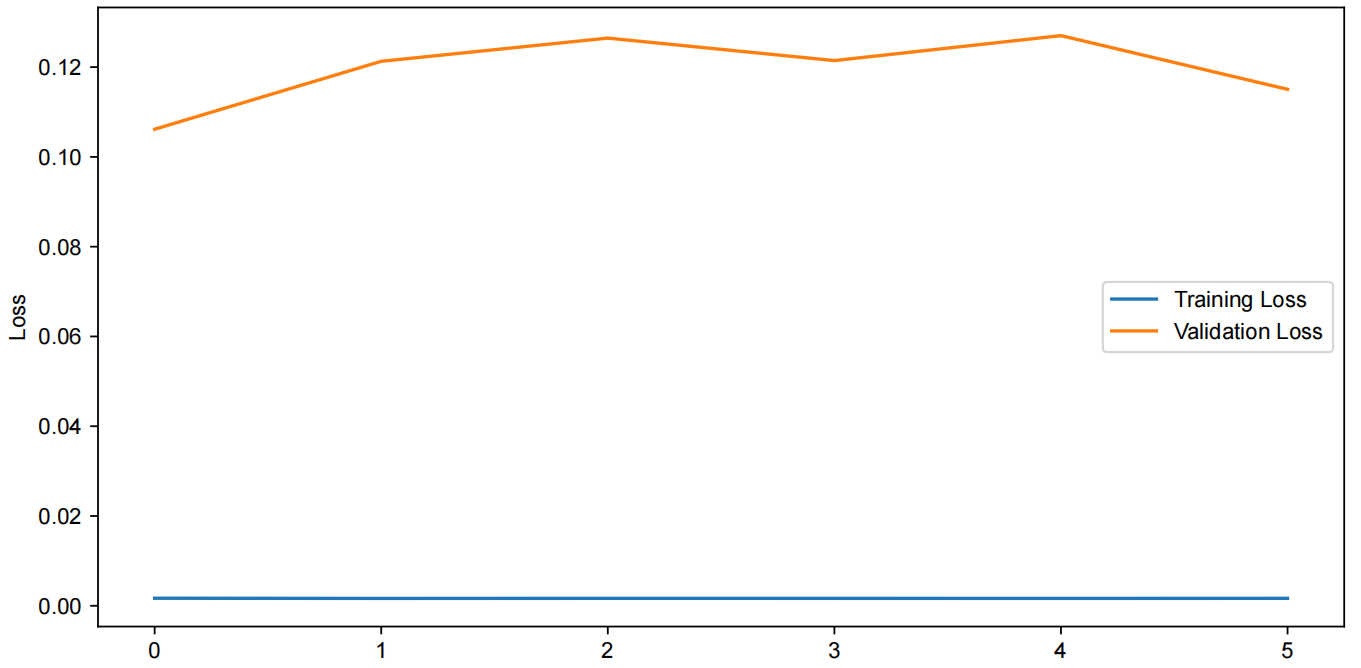
As shown in Figure 3 , the training and validation losses of the LSTM model converge well.

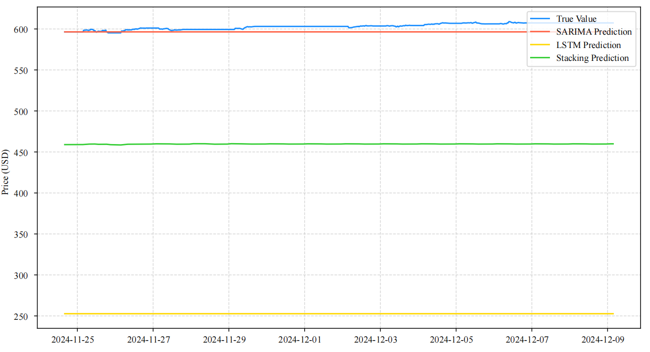
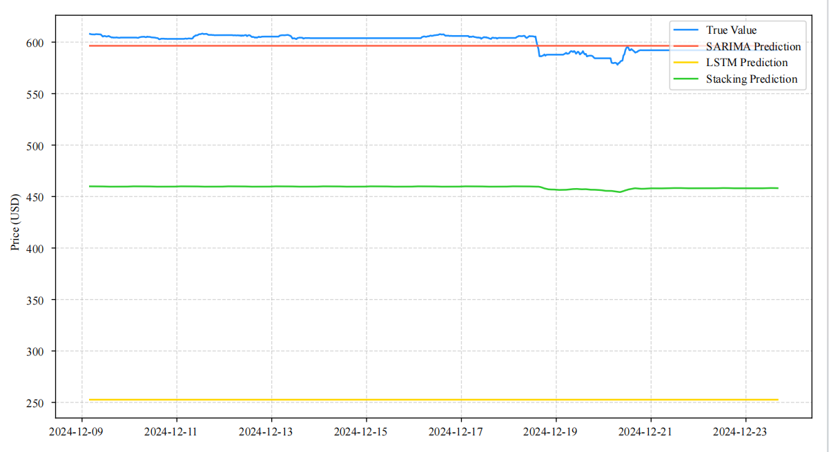
Figures 4 is the test set prediction comparison. Figure 5 is the validation set prediction comparison. the stacking model produces prediction curves that are closest to the actual values on both the validation set and the test set from December 9 to 23, 2024, outperforming Seasonal AutoRegressive Integrated Moving Average (SARIMA) and LSTM.

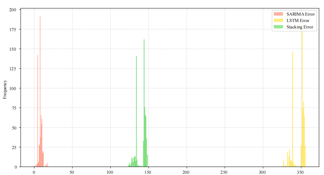
Figure 6 shows that the stacking model’s prediction errors are more concentrated in the low-value range, demonstrating both stability and accuracy. In terms of quantitative results, ARIMA (MSE = 0.1117), LSTM (MSE = 2.5359), dynamic weighting (MSE = 22.2479, MAE = 4.717), and stacking (MSE = 17.6145, MAE = 4.197) clearly reflect the performance differences. On the validation set, the stacking model achieves MSE = 7.6888 and MAE = 2.2708, both lower than those of dynamic weighting (MSE = 9.5823, MAE = 2.2257), confirming its advantage in error control.

4.2.  Results analysis and hypothesis testing

Trend analysis shows that ARIMA achieves errors of less than USD 0.5 during stable periods (October–November) but reaches USD 2.3 during volatile periods (December). In contrast, LSTM reduces the error to USD 1.2 in volatile periods but exhibits overfitting in stable periods with a deviation of USD 0.8. Stacking maintains consistently low errors in both stable (< USD 0.3) and volatile (< USD 1.0) periods, while dynamic weighting still records an error of USD 1.8 during volatile periods, indicating its lagging nature (Figure 5).

Indicator analysis further shows that stacking integration yields overall lower errors than dynamic weighting, with test set MSE (7.6888) still outperforming dynamic weighting (9.5823).

In hypothesis testing: first, the hybrid models outperform single models in overall accuracy (Figure 4, Figure 5, Figure 6). Stacking outperforms dynamic weighting (Figure 6). LSTM outperforms ARIMA in nonlinear volatile periods (Figure 4,Figure 6).

In summary, stacking consistently demonstrates the best performance across different volatility environments, while dynamic weighting is limited by its lagging effect during sudden market shocks.

5.  Conclusion

This study addresses the problem of forecasting short-term volatility of SPY during Federal Reserve interest rate cut cycles by constructing a hybrid LSTM-ARIMA model that integrates the strengths of ARIMA and LSTM. Dual integration strategies—dynamic weighting and stacking—are introduced to simultaneously capture the linear trends and nonlinear fluctuations of the market. The empirical analysis is based on 30-minute high-frequency data of the S&P 500 index, incorporating macroeconomic and market indicators such as the federal funds rate, the VIX index, and CPI as feature variables.

The results show that interest rate cut cycles significantly amplify SPY’s short-term volatility, with the expansion effect being most pronounced within 3–5 trading days following policy announcements. The hybrid model outperforms single ARIMA or LSTM models in both predictive accuracy and stability, with stacking integration demonstrating the best adaptability during policy shocks. In contrast, dynamic weighting, which relies on historical MSE, exhibits lagging effects under regime shifts. These findings are consistent with mainstream research that highlights the amplification of stock market volatility during interest rate cuts and the superiority of combined models over single models. Moreover, this paper makes a novel methodological contribution by paralleling dynamic weighting with stacking strategies in financial time series, applying K-means clustering for period-specific weight allocation, and thus proposing a new integration pathway and optimization approach that supplements empirical research and advances methodological innovation in financial volatility forecasting.

From a practical perspective, the findings provide valuable implications for investors, trading institutions, and risk management departments in addressing volatility during interest rate cut cycles. In the early stages of a rate cut cycle, LSTM signals can be leveraged to capture nonlinear fluctuation opportunities, while during stable periods, ARIMA signals offer robust guidance for identifying trend centers. When model prediction errors exceed a certain threshold, risk control measures should be triggered in time to guard against extreme events.

In terms of methodological optimization, future research may extend the time horizon to cover multiple economic cycles and incorporate multidimensional features such as trading volume, sentiment indices, and additional macroeconomic indicators to enhance explanatory power and robustness. For integration strategies, real-time regime recognition and online learning mechanisms could be introduced to improve the responsiveness of dynamic weighting, while nonlinear meta-models (e.g., XGBoost, Random Forest) may replace linear regression to enhance residual correction in stacking. Furthermore, Bayesian optimization and lightweight architectures could be employed to improve hyperparameter search and computational efficiency. This framework can also be extended to interest rate hike cycles, other asset classes, and cross-market volatility forecasting, offering broader applications for macroeconomic policy analysis and asset pricing research.

References

[1]. Kim, J. (2023) Interest Rate Cuts and Stock Market Volatility: Evidence From Global Monetary Cycles. Journal of Financial Economics, 148(2), 215-234.
[2]. Sâadaoui, F. & Rabbouch, H. (2024) Financial Forecasting Improvement With LSTM-ARFIMA Hybrid Models and Non-Gaussian Distributions. Technological Forecasting and Social Change, 198, 123539.
[3]. Saleti, S., Panchumarthi, L. Y., Reddy Kallam, Y., Parchuri, L. & Jitte, S. (2024) Enhancing Forecasting Accuracy With a Moving Average-Integrated Hybrid ARIMA-LSTM Model. SN Computer Science, 5, 704.
[4]. Petrozziello, A. (2022) Deep Learning for Complex Dynamic System Modeling: Advances and Applications. Journal of Computational Finance, 25(4), 33-58.
[5]. Hamiane, S., Ghanou, Y., Khalifi, H. & Telmem, M. (2024) Comparative Analysis of LSTM, ARIMA, and Hybrid Models for Forecasting Future GDP. Ingénierie des Systèmes d'Information, 29(3), 853-861.
[6]. Box, G. E. P. & Jenkins, G. M. (1970) Time Series Analysis: Forecasting and Control. Holden-Day.
[7]. Hochreiter, S. & Schmidhuber, J. (1997) Long Short-Term Memory. Neural Computation, 9(8), 1735-1780.
[8]. Breiman, L. (1996) Bagging Predictors. Machine Learning, 24(2), 123-140.
[9]. Hybrid ML Models for Volatility Prediction in Financial Risk Management (2025) Expert Systems With Applications, 252, 125078.
[10]. MacQueen, J. (1967) Some Methods for Classification and Analysis of Multivariate Observations. In L. M. LeCam & J. Neyman (Eds.), Proceedings of the Fifth Berkeley Symposium on Mathematical Statistics and Probability, 1, 281-297. University of California Press.
[11]. A Hybrid Approach of Wavelet Transform, ARIMA and LSTM Model for the Stock Index Futures (2023) Information Sciences, 640, 1456-1472.
[12]. Wolpert, D. H. (1992) Stacked Generalization. Neural Networks, 5(2), 241-259.
[13]. Michańków, J., Kwiatkowski, Ł. & Morajda, J. (2023) Combining Deep Learning and GARCH Models for Financial Volatility and Risk Forecasting. arXiv preprint, arXiv: 2310.01063.
[14]. Volatility Forecasting With Hybrid Neural Networks Methods for Risk-Controlled Strategy for Portfolio Allocation (2023) Expert Systems With Applications, 213, 120920.
Cite this article
Tian,W. (2025). Predictions of Short-Term Volatility in the U.S. Stock Market During Interest Rate Cut Cycles. Advances in Economics, Management and Political Sciences,241,96-105.
Data availability
The datasets used and/or analyzed during the current study will be available from the authors upon reasonable request.
Disclaimer/Publisher's Note
The statements, opinions and data contained in all publications are solely those of the individual author(s) and contributor(s) and not of EWA Publishing and/or the editor(s). EWA Publishing and/or the editor(s) disclaim responsibility for any injury to people or property resulting from any ideas, methods, instructions or products referred to in the content.
About volume
Volume title: Proceedings of ICFTBA 2025 Symposium: Global Trends in Green Financial Innovation and Technology
© 2024 by the author(s). Licensee EWA Publishing, Oxford, UK. This article is an open access article distributed under the terms and
conditions of the Creative Commons Attribution (CC BY) license. Authors who
publish this series agree to the following terms:
1. Authors retain copyright and grant the series right of first publication with the work simultaneously licensed under a Creative Commons
Attribution License that allows others to share the work with an acknowledgment of the work's authorship and initial publication in this
series.
2. Authors are able to enter into separate, additional contractual arrangements for the non-exclusive distribution of the series's published
version of the work (e.g., post it to an institutional repository or publish it in a book), with an acknowledgment of its initial
publication in this series.
3. Authors are permitted and encouraged to post their work online (e.g., in institutional repositories or on their website) prior to and
during the submission process, as it can lead to productive exchanges, as well as earlier and greater citation of published work (See
Open access policy for details).