1. Introduction

CAPM model is an equilibrium model of financial asset pricing established by William F Sharpe [1] and John Lintner [2] based on Markowitz's portfolio theory. The model provides the equilibrium price of risk assets as well as a description of the connection between risk and the return rate of risky assets in the equilibrium condition of the investment market.

While Chinese researchers just recently began studying the CAPM model, international academics have theoretically expanded and augmented it in a wide range of ways since it was first introduced. The CAPM model has drawn the interest of many academics with the formation and growth of China's securities market, and there has been much debate about whether it is suitable for the Chinese stock market.

The majority of current studies employ market composite indexes and some individual stock data as their study objects, and they group them using the conventional BJS approach [3]. However, this two-way regression method will have bias in the variable selection [4]. In addition to lessening the subjectivity of artificial selection and categorization, the research employing industry data from the stock market would also provide more thorough data. Further research and testing of the CAPM's efficacy in China's present capital market utilizing the most recent data are required due to the constant development of the country's stock market as well as the major changes in the number, size, trading system, and industry categorization of listed businesses.

As a result, an empirical study on the relationship between risk and return is conducted according to existing researches, the industry grouping method and the industry index data of the Chinese stock market in recent years. On the basis of that, it will be possible to investigate if the CAPM model is appropriate for the Chinese stock market and its features, as well as how the validity of the model's foundation in established Western markets would alter.

2. Methodology

2.1. Theoretical Model

According to Sharpe Lintner's concept, investors can borrow money at a rate of return free from risk. The most popular version of CAPM, which is also the standard form, is as follows:

Where \( E({R_{i}}) \) is the expected return on stock or portfolio \( i \) , \( {R_{f}} \) is the return on the risk-free asset, \( E({R_{m}}) \) is the expected return on the market portfolio, and \( {β_{i}}=\frac{cov({R_{i}},{R_{m}})}{Var({R_{m}})} \) is the market factor risk premium, which represents how sensitive stock return fluctuations are to changes in market portfolio returns.

Given that all assets have a fair chance of returning a profit, the realized rate of return on assets should match the projected rate of return [5]. Thus, if \( {ε_{i}} \) is introduced as a random error, The formula's expected form can be transformed into a random form by:

2.2. Data Selection and Processing

2.2.1. Sample Selection and Data Sources

The Chinese stock market started late and fluctuated greatly. The turmoil in China's stock market was especially severe when the global financial crisis broke out in 2008. The direction of the stock market has stabilized in recent years as China's financial industry has steadily grown and expanded. a 7-year sample span was chosen for this work, ranging from January 5, 2015, to December 31, 2021.

In addition, the 2021 edition of the Shenwan Industry Classification is used as the standard, and under which there are 31 first-class industries. As petroleum and petrochemical, environmental protection and beauty care are emerging industries, the data coverage range is less than one year. At the same time, due to the lack of data for some years of the coal industry on the official website of the Shenwan index, the above four industries are not included in the research scope After excluding the above industries, 27 industries in the Shenwan Industry Classification are used as research subjects, with data obtained from the Shenwan Index website [6].

Since the CSI 300 Index is a weighted index of 300 large, well run and liquid A-shares from the Shanghai and Shenzhen stock markets, it comprehensively reflects the market sentiment of the entire A-share market more comprehensively and has good market representativeness, the CSI 300 Index is used to represent the market portfolio and the data used are obtained from CSMAR database [7].

2.2.2. Determination of the Risk-free Rate

The rate of interest at which investors can borrow essentially risk-free is known as the risk-free rate of return. For research purposes, the one-year government bond interest rate is typically used by foreign academics as the risk-free interest rate for research. However, China has not yet achieved interest rate marketization at this stage, and although one-year treasury bonds have been issued, the interest rate of one-year treasury bonds varies greatly due to the difference between certificated and book-entry types and the phased issuance. Furthermore, the repurchase of government bonds is dominated by institutional investors, while a large part of the Chinese stock market is personal investment. Naturally, government bonds cannot be used as a risk-free interest rate selection criterion.

The main investment opportunities for individual investors are savings, stocks and treasury bonds, of which savings account for a large proportion and are generally considered risk-free. Through analysis of residential savings deposit rates and Treasury repo rates, etc., this paper selects the three-month bank term deposit rate as the risk-free rate, which undergoes six adjustments over the sample period as shown in the table below, taking the average of the three-month term deposit rates over the sample period and converting them to an average daily rate of 0.00447%. The data used is obtained from the Official website of the People's Bank of China [8].

Table 1: 2015/1/5-2021/12/31 Three-month benchmark interest rate of RMB deposits of financial institutions.

2.2.3. Calculation of Return on Assets

In general, the continuous compound rate of return approximates the normal distribution and has stronger statistical properties that can improve the smoothness of the time series. For this reason, the daily logarithmic rate of return in this study is determined using the continuous compound rate of return.

Where: \( {R_{it}} \) is the return of stock or portfolio \( i \) at moment \( t \) ; \( {P_{it}} \) is the price of stock or portfolio \( i \) at moment \( t \) ; \( {P_{i(t-1)}} \) is the price of stock or portfolio \( i \) at moment \( t-1 \) .

3. Test Methods and Empirical Results

A cross-sectional technique and time series test are utilized in combination, as opposed to the conventional BJS method. The primary distinction is that equities are split into 27 portfolios according to industry type rather than using the size of the beta value as a grouping factor.

3.1. Calculation of Industry Beta Coefficients and Risk-return Analysis

First, the sample period was divided into periods according to different durations and the time series estimation model was determined based on the analysis above as follows.

Where \( {R_{it}} \) is the return of the \( i \) th industry portfolio at time \( t \) ; \( {R_{mt}} \) is the return of the market index at time \( t \) ; \( {R_{ft}} \) is the risk-free return at time \( t \) ; \( {a_{i}}, {β_{i}} \) are the estimated parameters; \( {ε_{it}} \) is the estimated residuals.

Secondly, based on the above models, linear regressions with least-squares can produce beta coefficients for 27 industry portfolios at different times, for a total of 7128 data sets.

The findings indicate that all regression models have a P-Value of less than 0.01, which means that the models are very significant. Additionally, more than 99.8% of the beta coefficients are positive, demonstrating a strong positive linear link between the excess return beta of each industrial portfolio and the return of the market (CSI 300 Index Index). Therefore, it can be tentatively concluded that the beta coefficients could reflect the risk premium of the daily returns of each industry portfolio.

The same conclusion can be obtained by analyzing the results of each classification period. Thus, the following will not show the analysis process and results of each period in turn, but take the half year (121 trading days) period as an example. The sample period can be divided into a total of 14 intervals, with the specific dates for each interval as shown in the table below.

Table 2: Specific dates of each sample period.

For each industry, a \( {β_{ij}} \) was estimated at the sample interval using regression model (4), where \( i \) denotes the industry ( \( i \) =1，2，…27) and \( j \) denotes the period ( \( j \) =1，2，…，14). 378 \( {β_{ij}} \) coefficients are available for the 27 industries, as shown in the table below, with \( {β_{1}} \) ， \( {β_{2}} \) ，... ， \( {β_{16}} \) in the header of the table denoting the \( β \) coefficients for periods 1 to 16 respectively.

Table 3: Beta coefficients of each industry in different periods.

The j1-J27 in Table2 represent 27 different industries, which are Media, Power Equipment, Electronics, Real Estate, Textile & Apparel, Finance, Iron & Steel, Public Service, National Defense Military, Mechanical Equipment, Basic Chemical, Computer, Household Appliance, Construction Material, Architectural Decoration, Transportation, Automobile, Light, Commercial Retail, Social Service, Food & Beverage, Communication, Pharmaceutical & Biological, Banking, Non-Ferrous Metal, Comprehensive, Farming, Forestry, Husbandry & Fishing, respectively.

From Table 2, the largest beta coefficient is 1.5, it is the beta coefficient of the computer industry in the 10th period. The second-largest beta coefficient is 1.46 and the smallest beta coefficient is 0.10, followed by 0.17, they are the beta coefficients for Social Services, Utilities, and Construction & Decoration respectively for the 13th period, which is 2020-12-29-2021-06-30 when China is experiencing a new crown epidemic. When analyzing the performance of the sectors in that period cross-sectionally it is easy to observe that there is an overall trough in the beta coefficients of the sectors in that period, with 17 of them reaching their lowest beta in the sample period. However, there are also 2 sectors (social services and food and beverage) where the beta coefficients reached the highest in the sample period, such results suggested the differences in volatility brought about by the epidemic for different sectors.

3.2. Descriptive Statistical Analysis of the Obtained Beta Coefficients

The risk premium of a stock or portfolio in relation to the market is represented by the beta coefficient, which takes into account both systematic risk and market excess premium.

When \( β \gt 1 \) , the sector portfolio's risk exceeds the market risk, and the excess return surpasses the market excess return, indicating that the sector is more active than the entire market and that the return exceeds the market return. In contrast, \( β \lt 1 \) implies that the sector portfolio's risk is lower than the market risk and its excess return is lower than the market excess return, indicating that the sector is less active than the overall market and its return is lower than the market return.

Understanding the general state of the coefficients in Table 3 is necessary. The average \( β \) coefficients and standard deviations for each industry are calculated and ranked in order of average value from small to large as shown in Table 4.

Table 4: Mean and standard deviation of beta coefficients across industries.

Table 4 shows a total of ten industries with beta coefficients less than 0.9: Banking, Public Service, National Defence Military, Textile & Apparel, etc., all of which have underperformed the broader market on average over the seven years. On the contrary, the only industry with an average beta coefficient greater than 1.1 is Finance. Additionally, referring to Table 2, it is easy to discover that the industry's beta coefficient exceeds 1.1 for more than 75% of the time, indicating that the industry has not only outperformed the market on average, but also that its risk and return have been much greater than the broader market over the seven years, with consistently better performance in most periods.

Table 3 displays the standard deviation of the beta coefficients for each industry, with the minimum being 0.10 (banks) and the largest being 0.33 (construction and decoration). There are 13 industries with standard deviations of beta coefficients greater than 0.20 and more than 80% of industries have standard deviations of beta coefficients greater than 0.15, indicating that the beta coefficients of industry portfolios are not well stabilized. Only national defense military, basic chemical, automobile, pharmaceutical and biological, banking and other six industries have the standard deviation of beta coefficient less than 0.15. Therefore, the beta coefficients of the industries still vary considerably over time during these seven years. This demonstrates that the risk and reward performance of an industry varies widely over time.

3.3. CAPM Validity Testing

Based on the classic CAPM model, the following regression equation is used to evaluate if there is a positive linear relationship between the average portfolio return R and the beta coefficient.

Where: \( {\bar{R}_{p}} \) is the average return of the portfolio, \( {β_{p}} \) is the beta coefficient of each portfolio obtained in the time series; \( {γ_{0}} \) 、 \( {γ_{1}} \) are the estimated parameters and \( {ε_{p}} \) is the estimated residual.

First, based on the conventional CAPM, the following hypotheses are advanced:

H1: The average excess return \( {\bar{R}_{p}} \) of the asset portfolio and the beta coefficient \( {β_{p}} \) have a linear relationship. The grouping technique addresses the issues of measurement and selection bias, and it is anticipated that the average excess return of the portfolio should be linearly correlated with the beta coefficient, which is a key component of the conventional model.

H2: The intercept \( {γ_{0}}=0 \) indicating that the beta coefficient captures all risk-related characteristics and that residuals, price-to-earnings ratio, company size, dividend yield and the squared term of beta have no effect on the portfolio's performance.

H3: The value of slope \( {γ_{1}} \) should match the difference between the market portfolio's return and the risk-free rate. The slope of the conventional model \( {γ_{1}}={R_{mt}}-{R_{ft}} \) and \( {γ_{1}} \gt 0 \) .

Secondly, coordinate points ( \( {\bar{R}_{ij}} \) ， \( {β_{ij}} \) ) are obtained from the average rate of return \( {\bar{R}_{ij}} \) and \( {β_{ij}} \) coefficients of 27 industries in each time interval. These coordinates are utilized in regression analysis and significance testing. Table 5 displays the outcomes of the tests. Furthermore, scatter plots of the mean return \( {\bar{R}_{ij}} \) and \( {β_{ij}} \) coefficients are drawn in Figure 1. The horizontal and vertical axes indicate the \( {β_{ij}} \) coefficient and the mean return \( {\bar{R}_{ij}} \) for each industry portfolio over the sample period, respectively.

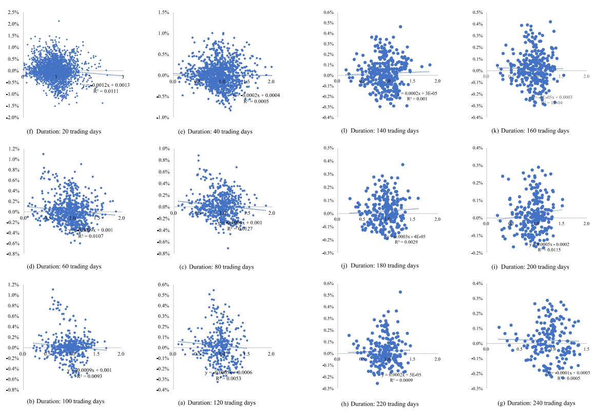
Figure 1: Correlation graph of beta coefficient & average return.

Figure 1 shows that the scatter plots of ( \( {\bar{R}_{ij}} \) ， \( {β_{ij}} \) ) data of different durations have no positive correlation, most of them show a certain negative correlation. To further test the correlation between the coefficients of average returns \( {\bar{R}_{ij}} \) and \( {β_{ij}} \) , the results of the linear regression equations are shown in the following table in ascending order of P-value.

Table 5: Regression models and statistical significance tests for mean returns and beta coefficients.

As shown in table 5, for the first 4 periods, the p-value of the F-test for the regression model is less than 0.05, indicating that the regression model is significant and that H1 may be accepted. However, \( {γ_{0}} \gt 0 \) , therefore assumption H2 should be rejected, which indicates that the portfolio returns are still influenced by other factors. Meanwhile, \( {γ_{1}} \lt 0 \) , therefore assumption H3 should also be rejected, which explains that the correlation between the average return \( {\bar{R}_{ij}} \) and \( {β_{ij}} \) coefficients is negative, and that the excess premium on the risk factor for the whole market is poorly explained. For most periods: the p-value of the F-test of the regression model is greater than 0.05 and therefore hypothesis H1 should be rejected, in other words, there is not a linear relationship between the average excess return \( {\bar{R}_{p}} \) and the beta coefficient \( {β_{p}} \) of the asset portfolio. In light of the above study, it is determined that the CAPM model is flawed.

4. Conclusion

From the results of the empirical analysis in this paper, the CAMP model is not applicable to China's stock market. Based on the findings of this paper's empirical investigation, the CAMP model cannot be applied to the Chinese stock market. Because there are very little association existing between stock returns and system risk on the stock market, systematic risk cannot explain changes in returns well. A significant portion of stock returns is influenced by non-systematic risk factors. Furthermore, contrary to what the CAPM theory predicts, there is no linear link between stock returns and systemic risk.

This paper reaches the same result as the majority of studies examining the applicability of the CAPM model to the Chinese market. This conclusion is also mandated by the state of the Chinese stock market at the moment. As an emerging market in a developing country, China's stock market is still very immature compared to stock markets in developed countries. Not only is the size small, many regulatory mechanisms and regulations are not sound, and there are major differences with Western countries, such as restrictions on short selling and a large number of illiquid shares, etc., which result in great differences between China's stock market and the market with strict hypothesis in CAPM model. In addition, there is more government intervention in the market in China, and the market is dominated by individual investors and lacks large institutional investors, all of which seriously affect the applicability of the CAPM in the Chinese market. In subsequent studies, research could be focused on more detailed empirical testing of the impact of non-systematic factors on the Chinese stock market revealed.

References

[1]. Sharpe, W.F. (1964), CAPITAL ASSET PRICES: A Theory of Market Equilibrium Under Conditions of Risk. The Journal of Finance, 19: 425-442.
[2]. Lintner, J. (1965) The Valuation of Risk Assets and the Selection of Risky Investments in Stock Portfolios and Capital Budgets. Review of Economics and Statistics, 47, 13-37.
[3]. Black F, Jensen MC,Scholes M. (1972) The Capital Asset Pricing Model: Some Empirical Test. Jensen MC. Studies in the Theory of Capital Markets. New York: Praeger Publishers Inc,1972:79-124.
[4]. Wang W, Tao S, Li J & Hou W. (2021). An empirical test of the validity of capital asset pricing model for Chinese enterprises. Journal of Huaibei Normal University (Natural Science edition) (04),23-31.
[5]. Ding L, Liu W (2013). An empirical test of capital asset pricing model in Shanghai stock market of China -- Based on dynamic grouping method. Journal of Zhongnan University of economics and Law (04), 101-109
[6]. Shenwan Index website (2021). http://www.swsindex.com/idx0130.aspx?columnid=8838
[7]. CSMAR database (2021). http://oldweb.csmar.com/Csmar.html
[8]. Official website of the People's Bank of China (2021). http://www.pbc.gov.cn/
Cite this article
Hou,Y. (2023). Empirical Test on CAPM Model of China's Stock Market by Industry Grouping. Advances in Economics, Management and Political Sciences,9,316-324.
Data availability
The datasets used and/or analyzed during the current study will be available from the authors upon reasonable request.
Disclaimer/Publisher's Note
The statements, opinions and data contained in all publications are solely those of the individual author(s) and contributor(s) and not of EWA Publishing and/or the editor(s). EWA Publishing and/or the editor(s) disclaim responsibility for any injury to people or property resulting from any ideas, methods, instructions or products referred to in the content.
About volume
Volume title: Proceedings of the 2nd International Conference on Business and Policy Studies
© 2024 by the author(s). Licensee EWA Publishing, Oxford, UK. This article is an open access article distributed under the terms and
conditions of the Creative Commons Attribution (CC BY) license. Authors who
publish this series agree to the following terms:
1. Authors retain copyright and grant the series right of first publication with the work simultaneously licensed under a Creative Commons
Attribution License that allows others to share the work with an acknowledgment of the work's authorship and initial publication in this
series.
2. Authors are able to enter into separate, additional contractual arrangements for the non-exclusive distribution of the series's published
version of the work (e.g., post it to an institutional repository or publish it in a book), with an acknowledgment of its initial
publication in this series.
3. Authors are permitted and encouraged to post their work online (e.g., in institutional repositories or on their website) prior to and
during the submission process, as it can lead to productive exchanges, as well as earlier and greater citation of published work (See
Open access policy for details).