


1. Introduction
The COVID-19 appeared in Wuhan, China in December 2019. Soon, it rapidly spread to the whole world within 3 months and was recognized as pandemic by WHO on March 11,2020. Apart from its negative impact on public health and social stability, it caused great pressure on the Chinese banking system, which is highly exposed to the negative effect of this pandemic.
Understanding financial connectedness is of interest in terms of understanding the financial risk triggered by COVID-19. In general, when an unexpected shock hits the economy, there would be less labor and consumption in the market, thus leading to the less active economy. Hence, most companies (including banks) would lose its equity with worried investors. Then, the banks would have to increase the leverage rate, not only mechanically because of the reduced equity value, but because they need to acquire more debt to fulfill their obligations, effectively transferring systemic risk among the banking system. With more mutual loan relationships within the system, more intricate networks would form. To be specific, this process indicates that the whole system would become highly interconnected and contagious as a risk in one bank can implicate other banks. This shows how the Chinese banking sector would be “too interconnected to fail.”
Understanding financial connectedness is also of interest in terms of finding the heterogeneity characteristic of the crisis during COVID-19 era. Generally speaking, the precursors of risk events would undermine the interconnection among the banking system and the spread of shock. This is because banks will better prepare in advance through risk control and diversification measures. For instance, the 2008 Global Financial Crisis followed a over-booming housing market, the 2013 Money Shortage in China followed a series of monetary policies, and the 2017 China–United States trade war followed a series of polices on trade intervention by Donald Trump. These crises were prompted by some beforehand policies and the "Grey Rhino" incidents, which acts as the indication of a highly risky period. However, the outbreak of COVID-19 was sudden and unpredictable. Hence, did this heterogeneity feature of COVID-19 impact the movement of the connectedness of Chinese banking system or its inner structure?
Though numerous relevant studies have been focused on the impact of COVID-19, its heterogeneity effect is still relatively elusive. In this context, our research aims (i) to initially quantify the impact of the COVID-19 on the connectedness of Chinese banking system, and (ii) to further explore the heterogeneity characteristic of the crisis during COVID-19 era by comparing it with previous crises. We focus our attention on Chinese banking system for the following reasons. First, China is the first country to experience the outbreak of COVID-19 and to recover from it, which offers us a complete period of the outbreak and recession of the pandemic to observe its impact. Second, the financial system in China is bank-dominated, which offers us a clear angle to understand the Chinese financial system stability [1].
For these purposes, we measure the volatility connectedness of 14 important banks in China over the last 12 years by using approach proposed by Diebold and Yilmaz [2]. The reason we choose volatility connectedness is that price volatility is distress-sensitive according to Diebold and Yilmaz [2]. That is, the higher the volatility, the riskier the stock or the market becomes. Thus, it is relatively effective for measuring the risk. As we started our research from 2008, when some Chinese banks are still not listed, we selected 4 state-owned banks, 7 commercial banks and 3 local banks. They account for 44% of the total bank assets and thus they can represent the Chinese banking system very well (as of Dec.31, 2021).
Our work has the following contributions: (i) Our work first covers the crises over the last 12 years and compares it with the ongoing crisis caused by pandemic, focusing on the Chinese banking system. This helps us understand the particularity of this ongoing crisis, and updates our understanding of it. (ii) As studies concerning with Chinese banking system focus more on the portfolio models and risk model, our work would fill the literature gap on measuring the connectedness of Chinese banking system by the volatility spillover network by Diebold and Yilmaz [2]. Furthermore, (iii) in our discussion of the crisis triggered by COVID-19, we divided banks into three categories based on its size and ownership (state-owned banks, joint-stock banks and local banks), in order to explore the differences in structural changes between them. This would offer us more precise observations for policymakers and other scholars.
The empirical findings show that the COVID-19 did impact the connectedness of Chinese banking system and its structure within the system, with the 14 Chinese banks highly interconnected especially during COVID-19 era. In addition, the highly connected and contagious status of Chinese banking system didn't stay long during COVID-19 era compared with previous crises. Moreover, we find a shock-passing path during the COVID-19 era: big banks deliver more shocks to the middle banks, and the middle banks send more shocks to small banks. At the same time, our work presents that state-owned banks, during COVID-19 era, were more contagious and the local banks were more vulnerable compared with their historical performance.
2. Literature Review
Our research here mainly links two strands of the literature. The first strand relates to the methodology of measuring connectedness of financial firms. The second strand is concerned with empirical findings, containing studies during the COVID-19 crisis.
2.1. Methodology on Measuring Connectedness
From a methodological perspective, different techniques have been applied. There are mainly two kinds of approaches based on its different model structure: (i) portfolio models and (ii) network models. For the portfolio models, it starts from measuring the risk of asset portfolio and then extend it to quantify systemic risk for an institution. According to the directions, models can be divided into two categories: (i) bottom-up and (ii) top-down methods. Using ∆CoVaR as a measure of systemic risk is the method from bottom to up, where ∆CoVaR represents the change in the value at risk of the financial system conditional on an institution being under distress relative to its median state [3]. Up-down models included vulnerability index (VI) [4], Shapley value [5], marginal expected shortfall (MES) [6], the component expected shortfall (CES) [7], and SRISK [8]. However, portfolio models only consider the individual connectedness between a financial institution and the financial system, independent of other financial institutions.
Hence, in order to take all the institutions in the system into account, some scholars introduced network models. First, network model mainly included three categories based on the type of the spillover:(i) mean spillover network, (ii) volatility spillover network and (iii) risk spillover network. For the mean spillover, the representative method is the Granger casual network proposed by Billio et al. [9]. For the volatility spillover network, Diebold and Yilmaz developed a network connectedness measurements with a generalized VAR framework from the spillover index approach of Diebold and Yilmaz based on vector autoregressive and variance decomposition [2,10,11]. For the risk spillover network, Hautsch et al. developed tail risk interdependence network using the realized systemic risk beta (total time-varying marginal effect of a firm's Value-at-risk (VaR) on the system's VaR) and LASSO method [12]. Similarly, Wang et al. proposed extreme risk spillover network based on CAViaR and the Granger causality risk test [13].
As studies concerning the Chinese banking system focus more on the portfolio models and risk model, our work would apply the volatility spillover network by Diebold and Yilmaz [2]. With its help, not only can we fill the literature gap on measuring the connectedness of Chinese banking system, but also, we would have a precise observation about volatility transmissions among main Chinese banks.
2.2. Empirical Findings on Connectedness
Since Diebold and Yilmaz proposed volatility spillover index and network, they are widely used in different context, covering various markets. For example, Diebold and Yilmaz examined daily volatility spillovers across US stock, bond, foreign exchange and commodities markets, and found that as the crisis intensified, so too did the volatility spillovers [10]. Diebold et al. applied the connectedness network to the commodity market [14]. Their result suggested clear clustering of commodities into groups that match traditional industry groupings in spite of some notable differences. Using Diebold and Yılmaz volatility diffusion network [2], Wang et al. investigated volatility connectedness in the Chinese banking system [15]. Their result showed that 14 Chinese commercial banks are highly interconnected and a positive (negative) rank correlation between size and from-connectedness (to-connectedness and net-connectedness) of banks. Apart form these literature, numerous scholars have expanded the scope of model application to other sectors, see Bubák et al., Antonakakis, Zhang and Wang, Maghyereh et al., Antonakakis and Kizys, Liow, Apergis et al [16-22].
One hot topic during ongoing pandemic is how the pandemic influenced the financial connectedness and systemic risk. Many scholars answer this question from different perspectives. For instance, from a global perspective, Rizwan et al. analyzed systemic risk of banking sectors of eight of the most COVID-19 affected countries, whose result showed that after a significant increase in systemic risk in all countries, it contains still at a high level except China [23]. Akhtaruzzaman et al. studied the occurrence of the financial contagion through financial and nonfinancial firms between China and G7 countries [24]. The result suggested a significant increase in conditional correlations between firms' stock returns. Another perspective is across-market. Amar et at. examined the spillovers and co-movements among commodity and stock prices major oil-producing and consuming countries [25]. The result showed that the spillovers reached their highest levels during the pandemic. And despite the existence of a significant interdependence among the world markets, Chinese and Saudi Arabian stock markets seem to be weakly integrated into the world market. Similar studies can be seen in Fasanya et al., Matos et al. and Corbet, Goodell, and Günay [26-28]
However, most literature only focus on the time period during pandemic, while ignoring the contrast of the connectedness between ongoing pandemic and previous crises and its heterogeneity effect. As this ongoing financial crisis is triggered by an unforeseen public health event, while most previous crises are caused by some predictable policies and the "Grey Rhino" incident, its particularity suggests that it might have different characteristics from previous crises. Thus, we would take connectedness during other big crises into account, which will be helpful for policymakers and people to get through this crisis. Furthermore, we would apply the methods on the Chinese banking system. Because China was recovering faster than others from this pandemic, and the financial system in China is bank-dominated, it really deserves our attention. However, few studies has analyzed it from the perspective of banking system. Thus, our study would explore the particularities and commonalities of this crisis by comparing the ongoing crisis with previous crises from the perspective of Chinese banking system.
The remainder of the paper is organized as follows. The third part deals with the research methods and data collection; the forth part focuses on empirical results and discussion; and the last part draws a conclusion and proposes some suggestions for future research.
3. Methodology and Data Collection
The methodology developed by Diebold and Yilmaz is widely used to analyze the connectedness of financial institutions [2,10]. In this paper, we use the VAR model and generalized variance decomposition to quantify connectedness of Chinese banks.
The idea of this method is to model the stock market volatility as an N-variable vector autoregression(VAR), and define the spillover as the sum of the forecast error variance due to other stocks' volatility.
3.1. Daily Range-based Realized Volatility
As has discussed in the section2, we choose the volatility connectedness as it is not widely applied in the study concerning the Chinese banking system. Following Garman and Klass [29], we estimate daily range-based realized volatility according to the formula:
\widetilde{σ}_{it}^{2}=0.511({H_{it}}-{L_{it}})-0.019[({C_{it}}-{O_{it}})({H_{it}}+{L_{it}}-2{O_{it}})-2({H_{it}}-{O_{it}})({L_{it}}{-O_{it}})]- 0.383{({C_{it}}-{O_{it}})^{2}} (1)
where {H_{it}} , {L_{it}} , {O_{it}} and {C_{it}} are, respectively, the logs of daily high, low, opening and closing prices for bank stock i on day t. Demirer et al. pointed out that, based on the fact that daily actual volatility is less sensitive to specific forms of microstructural noise and less susceptible to it, the index requires only four inputs per day, and it can be used in an efficient way through public data to calculate the actual volatility [30]. Then, we model the stock market volatility as an N-variable vector autoregression, and the detailed steps would be discussed in the next subsection.
3.2. Connectedness Measures
We now introduce our connectedness measures. We start with the pairwise directional connectedness, then move to total directional connectedness and total connectedness.
The pairwise directional is based on vector autoregression (VAR), where the forecast error decompositions (FEVD) are computed from a generalized VAR.
A reduced-form VAR model (Sims, 1981) is:
{y_{t}}=v+{A_{1}}{y_{t-1}}+{A_{2}}{y_{t-2}}+…+{A_{p}}{y_{t-p}}+{u_{t}} (2)
where is a N-dimensional vector of endogenous variables, is a N-by-N matrix, is a vector of i.i.d. error terms with zero mean. The VAR(p) can be casted in the companion VAR(1) form as follows:
{Y_{t}}=v+A{Y_{t-1}}+{U_{t}} (3)
where
{Y_{t}}≡( \begin{array}{c} {y_{t}} \\ {y_{t-1}} \\ ⋮ \\ {y_{t-p+1}} \end{array} ) , A≡[\begin{matrix}{A_{1}} & {A_{2}} & … & {A_{p-1}} & {A_{p}} \\ {I_{N}} & 0 & … & 0 & 0 \\ 0 & {I_{N}} & 0 & 0 & 0 \\ ⋮ & & ⋱ & ⋮ & ⋮ \\ 0 & 0 & … & {I_{N}} & 0 \\ \end{matrix}] , {U_{t}}≡( \begin{array}{c} {u_{t}} \\ 0 \\ ⋮ \\ 0 \end{array} ) (4)
If we assume the VAR(p) process is stable, then its moving average (MA) representation can be obtained by successive substitution for {Y_{t-i}} . Thus, it can be read:
{y_{t}}=A{(L)^{-1}}v+A{(L)^{-1}}{u_{t}}=A{(L)^{-1}}v+\sum _{i=1}^{∞}J{A^{i}}{J^{ \prime }}J{U_{t-i}}=μ+\sum _{j=1}^{∞}{Φ_{i}}{u_{t-i}} (5)
where J≡[{I_{N}},{0_{N×N(p-1)}}] is the selection matrix; A{(L)^{-1}}=\sum _{i=0}^{∞}Φ{L_{i}}=J{A^{i}}J for i=0, 1, … . Following Diebold and Yilmaz(2014), the H-step ahead generalized FEVD is:
d_{ij}^{H}=\frac{σ_{jj}^{-1}\sum _{h=0}^{H-1}{(e_{i}^{ \prime }{Φ_{h}}{Σ_{u}}{e_{j}})^{2}}}{\sum _{h=0}^{H-1}(e_{i}^{ \prime }{Φ_{h}}{Σ_{u}}{e_{j}})} (6)
where ∑ is the variance matrix of the vector of errors, {σ_{jj}} is the standard deviation of the error term of the {j^{th}} equation, and {e_{i}} is a vector with one on the {i^{th}} element and zero otherwise. Since the sum of elements in each row of the variance decomposition matrix is not equal to 1, we normalize each decomposition matrix element as:
\widetilde{d_{ij}^{H}}=\frac{d_{ij}^{H}}{\sum _{j=1}^{N}d_{ij}^{H}} (7)
where \widetilde{d_{ij}^{H}} is being a measure of the pairwise directional connectedness from VaR j to VaR i at horizon H.
Then, in order to analyze the bidirectional relationship between one bank to another bank, we calculate the net pairwise directional connectedness from bank {i^{th}} to bank {j^{th}} as:
C_{ij}^{H}=C_{j ← i}^{H}-C_{i ←j}^{H} , C_{j ← i}^{H} = \widetilde{d_{ji}^{H}} (8)
Then, based on the pairwise directional connectedness, we introduce three total directional connectedness indexes: (i) from-connectedness, (ii) to-connectedness and the (iii) net-connectedness. We use them to analyse the bidirectional relationship between one bank to other individual banks.
The from-connectedness to bank {i^{th}} is defined as:
{C_{i ←* }}=\sum _{j=1, j≠i}^{N}d_{ij}^{H} (9)
The to-connectedness from bank {j^{th}} is given by:
{C_{* ←j}}=\sum _{i=1, i≠j}^{N}d_{ij}^{H} (10)
The net-connectedness from bank {i^{th}} measures is:
C_{i}^{H}={C_{* ← i}}- {C_{i ← *}} (11)
Last, we calculate the total volatility connectedness index as the measurement of the average contribution of spillover from shocks across all variables to the total forecast error variance. In other words, it can be seen as the spillover of the whole system, and it's given by:
TCL(H) = \frac{\sum _{i,j=1;i≠j}^{N}d_{ij}^{H}}{\sum _{i,j=1}^{N}d_{ij}^{H}}=\frac{\sum _{i,j=1;i≠j}^{N}d_{ij}^{H}}{N} (12)
3.3. Data Collection
We apply the volatility spillover network to China's publicly-traded commercial banks for studying their volatility connectedness. Following Wang, Xie, Zhao and Jiang who investigated the systemic risk of China banking system using approach proposed by Diebold and Yilmaz, we use market data of China's publicly-traded commercial banks to construct the volatility spillover network [2,15]. The reason is that the China stock market has become quite efficient since its reform on market regulation after China joined WTO in 2001 [31]. Hence, public information, such as price, can effectively represent the market expectation on companies' future performance.
As of Jan 1, 2008, there were 14 banks listed, including 4 state-owned banks, 7 joint-stock banks and 3 local banks. They accounted for 44% of the total bank assets and thus they could represent the Chinese banking system effectively. Following above methodology, we collect daily high, low, opening and closing prices for 14 commercial banks during the period from Jan 1, 2008 to May 12, 2022. The data comes from Wind Info.
Table 1 shows the information of 14 commercial banks including their tickers, full names, corresponding abbreviations, asset size (as of Dec. 31 2021), and ranks of asset size. In the meantime, we also list the total assets of the above banks and all banks. We find that stated-owned banks have largest asset size, followed by joint-stock commercial banks and local banks.
Table 1: 14 China's publicly-traded commercial banks with tickers, abbreviations, asset size, and ranks of asset size.
Ticker | Bank | Abbr. | Asset Size | Rank of Asset Size |
Panel A: State-owned commercial banks | ||||
601398.SH | Industrial and Commercial Bank of China Ltd. | ICBC | 35171.3 | 1 |
601939.SH | China Construction Bank | CB | 30254.0 | 2 |
601988.SH | Bank of China | BCHINA | 26722.4 | 3 |
601328.SH | Bank of Communications | BCOM | 11665.8 | 4 |
Panel B: Joint-stock commercial banks | ||||
600036.SH | China Merchants Bank | CMB | 9249.0 | 5 |
601166.SH | Industrial Bank | IB | 8603.0 | 6 |
600000.SH | Shanghai Pudong Development Bank | SPDB | 8136.8 | 7 |
601998.SH | China CITIC Bank | CCB | 8042.9 | 8 |
600016.SH | China Minsheng Banking Corp., Ltd. | MB | 6952.8 | 9 |
000001.SZ | Ping An Bank | PAB | 4921.4 | 10 |
600015.SH | Huaxia Bank | HB | 3676.3 | 11 |
Panel C: Local banks | ||||
601169.SH | Bank of Beijing | BB | 3059.0 | 12 |
002142.SZ | Bank of Ningbo | NINGB | 2015.6 | 13 |
601009.SH | Bank of Nanjing | NANB | 1748.9 | 14 |
Total asset size of the above banks | 160219.1 | |||
Total asset size of the all banks | 357900.0 | |||
Ratio | 0.448 | |||
Note: They are classified into three types according to their ownership: (i) state-owned commercial banks, (ii) joint-stock commercial banks, and (iii) local banks. In each ticker, "SH" ("SZ") represents that a commercial bank's stock is traded on the Shanghai (Shenzhen) stock exchange. Asset Size are in billions Chinese yuan (CNY) as of 31 December 2021.
4. Result
In this section, we offer our empirical results. First, we present the static analysis on the connectedness findings during three sub-periods: (1) 2019, before the COVID-19 era; (2) 2020, first year of the COVID-19 era; (3) 2021, second year of the COVID-19 era. Here, compared with the economic growth rate in the 2020 quarter, the GDP in the four quarters of 2021 increased by 18.3%, 7.9%, 4.9% and 4.0% year-on-year respectively. Hence, we can state that China's economy has partly recovered in 2021 compared to 2020 perhaps due to effective anti-epidemic policies.
Then, based on the dynamic connectedness measures proposed by Diebold and Yilmaz, we build a rolling estimation to capture the complete movement of the connectedness of the whole banking system and banks of different ownership. In the same subsection, we also explore the uniqueness of this crisis pushed by COVID-19, by comparing the COVID-19 era with previous crises.
4.1. Static Estimation of the Chinese Banking Network
Here, we estimate realized volatility VAR's of 14 Chinese commercial banks using the methodology as described in Section 3. Then we compute variance decompositions and corresponding connectedness measures at horizon H = 12, using the estimated VAR parameters.
The connectedness in 2019, 2020 and 2021 appears as Table 2-4. First, the central 14x14 area is divided into 3x3 shares according to the bank's shareholding attributes, namely state-owned banks, joint-stock banks, and local banks. Second, the diagonal elements, the own connectedness, tend to be the largest individual elements of the table. In addition, the own connectedness of three state-owned banks is noticeably less than that of other two kinds if banks. Here the own connectedness measures the volatility shock to the bank coming from itself, that is the internal shock. Third, as for the off-diagonal elements, they measure the external shock from another bank or to another bank.
The total direct connectedness deg”ee o' "from others" is the sum of the pairwise connectedness degrees of other banks in the system to a certain bank, which reflects the total risk spillover effect of other banks in the system to this bank, the depth of which can be regarded as an indicator to measure the “vulnerability” of each bank. Similarly, the total direct connectedness degree of “to others” is the sum of the pairwise connectedness degree of a bank to other banks in the system, reflecting the relationship between this bank and other banks in the system. The total risk spillover effect of a bank shows the bank's ability to spread volatility shocks and risks and can be seen as an indicator of the “contagiousness” of individual banks. Hence, it can be concluded that a bank of high contagiousness is likely to high vulnerability.
Let's start with table 2-4. First, we can find the total connectedness in 2019 and 2020 is similar, respectively 85.4% and 87.5%, and dropped to 69.2% in 2021. This means that the banks were highly interconnected in the first two years, but became not so interconnected in 2021 when the pandemic was relatively controlled. Hence, this implies that the system is well integrated, with only a around 15% change in the system, which is the result of idiosyncratic shocks in other markets. Besides, the difference of the total connectedness in 2020 and 2021 implies that the COVID-19 did impact the banking connectedness a lot. When the economy recovered in 2021, the market value of banks increased, hence reducing the leverage ratios of banks and less mutual loan relationships within the system. In addition, with liquidity provided to the market by the central bank, the amount of loan traded among banks could decrease, thus naturally reducing the connectedness within the banking system.
The reason why total connectedness was also high in 2019 is that it was partly influenced by the US-China trade dispute. In June 2018, the US announced that it would impose a 25% punitive tariff on 34-billion dollars of Chinese goods, which had a heavy impact on the Chinese stock markets, firstly influencing the sectors which export products on the US tariff lists and then the other sectors with direct or indirect connections to the banking system, since banks are the primary source of financing for businesses. However, despite tariffs on China that began in Trump's term still continue to 2021, the following released information exhibited much weaker impacts and only results in sector specific risk spillovers, like communication and computer sectors [32]. Hence, US-China trade dispute had limited impact on increasing total connectedness in 2021.
Table 2: Static connectedness table, 2019, before COVID-19.
ICBC | CB | BCHINA | BCOM | CMB | IB | SPDB | CCB | MB | PAB | HB | BB | NINGB | NANB | FROM | |
ICBC | 13.5 | 9.8 | 8.9 | 6.7 | 2.1 | 5.6 | 4.3 | 7.9 | 9.4 | 5.0 | 9.2 | 8.9 | 3.0 | 5.6 | 86.5 |
CB | 6.1 | 11.7 | 9.0 | 5.4 | 2.9 | 4.5 | 5.5 | 8.4 | 10.9 | 6.3 | 10.7 | 10.2 | 3.4 | 5.2 | 88.3 |
BCHINA | 7.1 | 8.6 | 13.0 | 9.5 | 3.2 | 3.5 | 4.8 | 7.6 | 9.3 | 5.0 | 9.1 | 9.9 | 3.0 | 6.3 | 87.0 |
BCOM | 5.9 | 9.2 | 9.1 | 12.1 | 3.5 | 2.9 | 3.3 | 9.0 | 10.6 | 5.6 | 11.2 | 10.6 | 4.0 | 3.0 | 87.9 |
CMB | 3.4 | 8.3 | 7.0 | 4.8 | 19.0 | 7.0 | 9.0 | 3.9 | 7.0 | 8.3 | 7.0 | 5.7 | 3.9 | 5.6 | 81.0 |
IB | 5.0 | 7.8 | 8.0 | 5.6 | 2.4 | 11.7 | 6.8 | 7.4 | 8.0 | 5.9 | 8.4 | 7.0 | 7.0 | 8.9 | 88.3 |
SPDB | 3.8 | 7.9 | 6.8 | 3.6 | 3.4 | 6.1 | 11.7 | 8.5 | 8.5 | 8.4 | 8.8 | 8.0 | 5.8 | 9.0 | 88.3 |
CCB | 2.1 | 8.9 | 7.2 | 4.4 | 1.9 | 1.3 | 3.3 | 15.1 | 13.1 | 7.5 | 14.5 | 13.5 | 4.7 | 2.5 | 84.9 |
MB | 3.3 | 9.4 | 8.3 | 4.8 | 2.0 | 2.7 | 4.8 | 11.6 | 13.2 | 7.1 | 13.1 | 12.6 | 3.3 | 3.9 | 86.8 |
PAB | 4.5 | 7.7 | 6.9 | 3.7 | 2.8 | 4.8 | 6.6 | 8.2 | 7.9 | 12.5 | 8.6 | 7.6 | 9.6 | 8.5 | 87.5 |
HB | 3.4 | 9.3 | 7.9 | 5.1 | 1.9 | 2.3 | 4.0 | 11.8 | 12.9 | 7.0 | 14.1 | 13.0 | 3.9 | 3.3 | 85.9 |
BB | 4.2 | 9.3 | 8.9 | 5.3 | 2.0 | 2.6 | 5.2 | 10.4 | 12.4 | 6.5 | 12.5 | 13.2 | 3.1 | 4.2 | 86.8 |
NINGB | 3.3 | 5.2 | 6.0 | 2.7 | 2.8 | 5.9 | 4.5 | 6.4 | 5.4 | 6.2 | 6.0 | 5.8 | 30.5 | 9.4 | 69.5 |
NANB | 6.0 | 6.9 | 9.1 | 5.0 | 1.7 | 7.6 | 7.3 | 6.6 | 6.7 | 6.2 | 7.3 | 6.5 | 9.6 | 13.5 | 86.5 |
TO | 58.2 | 108.4 | 103.1 | 66.5 | 32.6 | 56.9 | 69.4 | 107.7 | 122.0 | 84.9 | 126.5 | 119.2 | 64.2 | 75.3 | 85.4 |
NET | -28.3 | 20.1 | 16.1 | -21.3 | -48.4 | -31.4 | -18.9 | 22.8 | 35.2 | -2.6 | 40.6 | 32.5 | -5.3 | -11.2 |
Table 3: Static connectedness table, 2020, first year of the COVID-19 era.
ICBC | CB | BCHINA | BCOM | CMB | IB | SPDB | CCB | MB | PAB | HB | BB | NINGB | NANB | FROM | |
ICBC | 12.0 | 9.5 | 8.4 | 8.6 | 4.6 | 6.9 | 8.8 | 7.4 | 8.5 | 3.5 | 7.3 | 7.8 | 3.3 | 3.3 | 88.0 |
CB | 9.3 | 9.2 | 7.7 | 8.6 | 4.7 | 6.7 | 8.3 | 8.7 | 8.6 | 3.8 | 7.7 | 8.5 | 4.4 | 3.7 | 90.8 |
BCHINA | 9.3 | 7.7 | 13.4 | 11.1 | 2.4 | 5.9 | 9.8 | 5.9 | 9.7 | 2.7 | 6.7 | 7.9 | 3.2 | 4.2 | 86.6 |
BCOM | 7.9 | 7.0 | 10.1 | 11.9 | 3.3 | 6.1 | 8.6 | 9.5 | 9.3 | 3.4 | 6.6 | 8.4 | 3.6 | 4.3 | 88.1 |
CMB | 6.6 | 7.4 | 3.3 | 5.9 | 13.7 | 11.1 | 5.4 | 6.9 | 6.0 | 7.2 | 7.9 | 7.8 | 7.0 | 4.0 | 86.3 |
IB | 7.7 | 9.2 | 5.4 | 6.1 | 7.4 | 13.4 | 6.4 | 7.5 | 6.6 | 6.1 | 7.1 | 6.0 | 6.5 | 4.7 | 86.6 |
SPDB | 7.3 | 6.6 | 7.9 | 8.6 | 3.6 | 5.7 | 10.5 | 9.7 | 9.4 | 3.3 | 7.9 | 10.0 | 5.0 | 4.6 | 89.5 |
CCB | 6.6 | 6.6 | 5.2 | 7.9 | 5.4 | 6.2 | 6.5 | 16.2 | 8.0 | 3.4 | 7.0 | 9.3 | 5.5 | 6.1 | 83.8 |
MB | 7.2 | 6.7 | 8.4 | 9.7 | 3.5 | 5.2 | 9.2 | 9.8 | 10.6 | 3.5 | 8.2 | 9.6 | 4.0 | 4.4 | 89.4 |
PAB | 5.6 | 7.6 | 3.7 | 5.1 | 6.9 | 11.1 | 4.7 | 8.9 | 6.5 | 13.9 | 6.9 | 6.1 | 8.8 | 4.3 | 86.1 |
HB | 8.1 | 6.9 | 8.6 | 9.7 | 3.9 | 5.8 | 8.4 | 10.1 | 9.1 | 3.6 | 9.1 | 8.6 | 4.5 | 3.8 | 90.9 |
BB | 7.2 | 6.0 | 6.3 | 8.4 | 4.6 | 5.4 | 8.3 | 12.1 | 8.6 | 3.3 | 8.9 | 12.3 | 5.2 | 3.5 | 87.7 |
NINGB | 5.0 | 6.5 | 5.1 | 5.9 | 7.4 | 9.3 | 6.2 | 5.4 | 7.0 | 7.6 | 8.1 | 6.7 | 15.7 | 4.2 | 84.3 |
NANB | 5.5 | 6.9 | 4.5 | 4.3 | 6.5 | 7.4 | 6.5 | 9.5 | 6.5 | 3.9 | 5.8 | 5.1 | 14.1 | 13.5 | 86.5 |
TO | 93.3 | 94.4 | 84.7 | 99.9 | 64.4 | 92.8 | 97.1 | 111.2 | 103.8 | 55.2 | 96.0 | 101.7 | 75.1 | 55.0 | 87.5 |
NET | 5.4 | 3.6 | -1.9 | 11.8 | -21.9 | 6.2 | 7.5 | 27.5 | 14.4 | -30.9 | 5.2 | 14.0 | -9.2 | -31.5 |
Table 4: Static connectedness table, 2021, second year of the COVID-19 era.
ICBC | CB | BCHINA | BCOM | CMB | IB | SPDB | CCB | MB | PAB | HB | BB | NINGB | NANB | FROM | |
ICBC | 21.7 | 10.3 | 7.1 | 6.0 | 4.7 | 9.6 | 4.9 | 9.7 | 6.3 | 3.0 | 1.1 | 6.2 | 4.5 | 5.0 | 78.3 |
CB | 10.2 | 23.5 | 3.7 | 3.6 | 5.3 | 9.1 | 7.1 | 13.6 | 6.1 | 3.1 | 0.6 | 3.2 | 3.6 | 7.0 | 76.5 |
BCHINA | 8.3 | 4.5 | 41.3 | 8.1 | 2.8 | 4.9 | 4.9 | 4.2 | 4.3 | 2.6 | 1.5 | 4.5 | 3.8 | 4.2 | 58.7 |
BCOM | 8.3 | 5.3 | 3.4 | 41.6 | 4.2 | 4.0 | 4.9 | 8.4 | 2.8 | 1.4 | 1.3 | 5.5 | 5.1 | 3.8 | 58.4 |
CMB | 5.6 | 8.3 | 2.8 | 3.4 | 27.2 | 9.2 | 6.0 | 4.6 | 4.0 | 5.1 | 1.6 | 5.7 | 7.7 | 8.8 | 72.8 |
IB | 5.1 | 7.7 | 2.5 | 0.6 | 5.7 | 21.3 | 11.6 | 15.8 | 4.1 | 5.9 | 0.6 | 6.4 | 4.5 | 8.2 | 78.7 |
SPDB | 5.9 | 7.2 | 3.0 | 5.2 | 3.4 | 8.2 | 23.1 | 19.5 | 5.0 | 4.0 | 0.7 | 3.6 | 3.7 | 7.5 | 76.9 |
CCB | 7.4 | 9.6 | 3.9 | 6.3 | 3.2 | 7.3 | 12.2 | 29.4 | 6.5 | 1.7 | 1.1 | 2.9 | 2.6 | 5.9 | 70.6 |
MB | 8.2 | 5.7 | 3.3 | 5.4 | 4.9 | 5.6 | 4.2 | 13.5 | 27.6 | 3.2 | 1.6 | 9.0 | 1.6 | 6.2 | 72.4 |
PAB | 5.5 | 5.1 | 0.7 | 3.3 | 5.2 | 10.2 | 3.9 | 12.1 | 8.6 | 28.1 | 0.5 | 5.7 | 7.1 | 4.0 | 71.9 |
HB | 3.3 | 3.6 | 3.7 | 5.2 | 2.4 | 1.8 | 4.2 | 5.1 | 2.8 | 1.7 | 58.8 | 2.9 | 2.9 | 1.5 | 41.2 |
BB | 4.1 | 6.1 | 3.3 | 5.8 | 6.3 | 10.0 | 2.7 | 8.5 | 7.3 | 4.9 | 0.7 | 30.1 | 3.7 | 6.4 | 69.9 |
NINGB | 6.2 | 6.7 | 4.0 | 5.4 | 8.2 | 6.8 | 5.5 | 2.8 | 2.4 | 8.9 | 7.3 | 4.0 | 26.2 | 5.7 | 73.8 |
NANB | 4.2 | 6.5 | 7.0 | 5.9 | 8.8 | 11.0 | 1.9 | 2.7 | 2.4 | 4.3 | 0.7 | 7.5 | 6.7 | 30.6 | 69.4 |
TO | 82.3 | 86.6 | 48.4 | 64.2 | 65.2 | 97.9 | 74.0 | 120.4 | 62.6 | 49.8 | 19.2 | 67.1 | 57.6 | 74.2 | 69.2 |
NET | 4.0 | 10.1 | -10.3 | 5.8 | -7.6 | 19.2 | -2.9 | 49.8 | -9.8 | -22.1 | -22.0 | -2.8 | -16.2 | 4.8 |
Note for Table2-4: The ij-th entry of the upper-left 14x14 firm submatrix gives the ij-th pairwise directional connectedness; i.e., the percent of 12-day-ahead forecast error variance of firm i due to shocks from firm j. The rightmost (“FROM”) column gives total directional connectedness (from); i.e., row sums (“from all others to i”). The bottom (“TO”) row gives total directional connectedness (to); i.e., column sums (“to all others from j “). The bottom-most (“NET”) row gives the difference in total directional connectedness (to-from). The bottom-right element (in boldface) is total connectedness (mean “from” connectedness, or equivalently, mean “to” connectedness).
Second, with reference to the from-connectedness, we find a notable decline among all the banks in 2021 after they maintained at a similar level (80%-90%) in 2020 and 2021. To be specific, nearly all the banks had a from-connectedness above 80% in the first two years, while that of most banks was dropped below 80% in 2021, and some of them, including Bank of China, Bank of Communications and Huaxia bank, even showed a lower from-connectedness below 60%. This means that the volatility shock received from other banks dropped when the covid-19 was relatively controlled in 2021.
Then, the second-to-last row of the tables represents to-connectedness of 14 banks, which is more various than from-connectedness. Unlike from-connectedness, to-connectedness of different banks differed greatly. In 2019, except Nanjing Bank, all the banks' from-connectedness are 80%-90%, while the to-connectedness ranges from a minimum of 32.6% for China Merchants Bank to a maximum of 126.5% for Huaxia Bank. As shown in table 5, where we list the variance of the to-connectedness and from-connectedness in three sub-periods, the variance of from-connectedness is lower than that of to-connectedness in all the sub-periods.
At the same time, the change of to-connectedness also followed a different pattern from from-connectedness. Take the example of four national banks, a great increase (about 30%) of to-connectedness of ICBC and BCOM can be observed from 2019 to 2020, while that of the other two national banks dropped by around 15%. From 2020 to 2021, despite to-connectedness of all four banks dropped, BCHINA and BCOM decreased even more, almost three times as high as that of the other two. The explanation is that the size of volatility issued by one bank can be quite various with the large range (93.9%), but would be disturbed evenly across other banks. To be more specific, the size of volatility shocks sent to others would depend on the content of inter-bank transactions, which varied in different transactions. Similar findings can be seen in other markets, like Eurozone banking sector and US financial institutions [33].
Apart from that, another notable fact (shown in table 5) is that the variance of from-connectedness was only 24.3 in 2019 and 4.7 in 2020, while it rose to 103.6 in 2021. The lower figure in 2020 means that crisis led to an even distribution of volatility shocks across banking system, while the high variance of “from-connectedness” in 2021 suggests that there exists marked differences, or some special cases, in risk-sharing among different banks. To be specific, the figure for Huaxia Bank was extremely lower, with only 41.2%, in comparison with other figures which were mostly around 70%. As for to-connectedness, the lowest variance appears in 2020. This means when an external shock hit the banking system, most banks increased their to-connectedness to others together, thereby leading to a similar to-connectedness. When a bank gets hit, the best strategy is to borrow money from banks with lower risk. Hence, the banks which received little shocks in the past would have to help other banks, and thus absorbed more shocks until every bank had similar level of connectedness.
Table 5: Variance of the To-connectedness and From-connectedness in Three Sub-periods.
2019 | 2020 | 2021 | |
to-connectedness | 847.8 | 327.6 | 576.9 |
from-connectedness | 24.3 | 4.7 | 103.6 |
Forth, table 2-4 also show us the net-connectedness. When the net value is positive, it indicates that this bank is a volatility emitter (emits more volatility than it receives). When the net value is negative, it indicates that this bank is a volatility receiver(receive more volatility than it receives). After comparing three sub-periods, we find the important role COVID-19 plays in the transmission of volatility. For instance, many banks turn to a volatility emitter from a volatility receiver during COVID-19 era, including ICBC (from -28.3% to 5.4%), Bank of Communications (from -21.3% to 11.8%), Industrial Bank (from -31.4% to 6.2%) and Shanghai Pudong Development Bank (from -18.9% to 7.5%). In the same time, we also find that the increase of net-connectedness of China Merchants Bank (from -48.4% to -21.9%) and China CITIC Bank (from 22.8% to 27.5%), while the decrease of net-connectedness is seen among small banks, including China Minsheng Banking, Ping An Bank, Huaxia Bank, Bank of Beijing, Bank of Ningbo and Bank of Nanjing. This indicates during the pandemic, many big banks turned to send more volatility shock to the banking system, while small banks turned to a volatility receiver. This highlights the “too-big-to-fail” characteristic of Chinese banking system.
Table 6: Pairwise connectedness means of banks of different ownership.
state-owned bank | joint-stock bank | local bank | |
2019 | |||
state-owned banks | 7.9 | 6.5 | 6.1 |
joint-stock bank | 6.0 | 6.8 | 7.0 |
local bank | 6.0 | 6.3 | 6.5 |
2020 | |||
state-owned banks | 8.8 | 6.6 | 5.2 |
joint-stock bank | 7.0 | 6.8 | 6.2 |
local bank | 6.0 | 7.1 | 6.5 |
2021 | |||
state-owned banks | 6.6 | 4.9 | 4.7 |
joint-stock bank | 4.9 | 5.7 | 5.2 |
local bank | 5.4 | 5.4 | 5.7 |
Fifth, in order to dig the inner structure of connectedness within the system, we present the average of the pairwise connectedness of banks of different ownership in table 6. Here, we only calculate the means of off-diagonal elements, hence to get the transmission that only includes external shocks. By this way we can focus on the spread of the volatility shocks between different banks. Initially, with reference to shocks from state-owned banks, when the pandemic started, state-owned banks delivered more shocks (7%) to joint-stock banks, and joint-stock banks delivered more shocks (7.1%) to local banks. This presents a shock-passing path during the COVID-19 era, with big banks passing shocks to the middle banks, and the middle banks passing shocks to small banks. In addition to this, we found that local banks sent the most shocks to joint-stock banks, 7%, 6.2% and 5.2% respectively in three sub-periods. This means that joint-stock banks were the biggest cause of vulnerability of local banks, and local banks were also the biggest source of vulnerability of joint-stock banks at the same time. These two findings imply two notable shock-passing relationships within Chinese banking system: state-owned banks are tightly connected to joint-stock banks, and joint-stock banks are tightly connected to local banks, while the shock-passing path between state-owned banks and local banks is not obvious.
4.2. Dynamic Estimation of the Chinese Bank Network
In order to better investigate the spillover dynamics, we characterize the Chinese banking network dynamically by progressing from macro to micro in this sub-section. First, by using the rolling estimation with a 300-day window, we start with a dynamic analysis with the total connectedness of the same 14 banks mentioned in the earlier section. Then, we move to see the total connectedness of banks with different ownership, and characterize the structural change over time.
4.2.1. Total Connectedness
In figure 2 the total connectedness of Chinese banking system form 2008 to 2022 is presented. As we can see, the total volatility connectedness index has varied over time, ranging between 92% in 2015 and 55% in the beginning of 2022.
To start with, there are four big cycles across last 12 years. The first one lasted from 2008 to 2011, and the total connectedness fluctuated greatly. In September 2008, Lehman Brothers filed for bankruptcy protection, triggering a global financial crisis. Extreme risks were transmitted to the Chinese financial market through the interconnection channels of international financial markets and investor sentiment contagion channels, resulting in a sudden jump in the total connectedness to more than 90%. At the end of 2008, China launched the "Four Trillion Plan" (stimulating shadow banking) to stimulate the national economy hit hard by the international financial crisis. The ample liquidity increased the risk spillover effect between financial markets, and the total connectedness rose sharply again. In 2010, under the superposition of the European debt crisis and the second round of quantitative easing policy in the United States, the total connectedness continued to climb to a high of 87% [34].
In the second cycle, from 2013 to 2014, the total connectedness surged to 85% because of the "money shortage" in 2013. In June 2013, due to the withdrawal of the quantitative easing policy by the United States, a large influx of international hot money fled at the beginning of the year, coupled with the strengthening of regulatory policies, the growth rate of my country's money supply fell month-on-month, causing a "money shortage" event. Moreover, as the central bank issued 2 billion yuan of central bank bills on schedule, instead of using the short-term liquidity adjustment tool (SLO) as expected by the market. As a result, some banks had to cancel the preferential loan interest rate, leading to an increasing liquidity risk and a high systemic risk in the financial system.
The third cycle, from 2015 to 2017, was caused by an enhanced government regulation. In the first half of 2015, the China Securities Regulatory Commission imposed penalties on some securities companies that violated regulations in financing business and conducted large-scale inspections on the rest of the securities companies, which triggered extreme panic in the market over high-leverage funds and the regulatory authorities clean-up of the financing business. Hence, systemic risks in financial institutions rose, causing the total connectedness increased dramatically to 93%.
The last cycle, from 2018 to 2022, started with the US-China trade dispute after U.S. President Donald Trump began setting tariffs and other trade barriers on China, exacerbating the linkage of volatility among financial markets, and the total connectedness once climbed [32]. Then the outbreak of the covid-19 epidemic in December 2019 triggered panic contagion by viral contagion, which in turn brought about cross-market contagion of financial risks, leading to another sharp jump in the total connectedness, and it continues to the end of 2021. In April 2022, owing to withdrawal freezing in some China's Village Bank, the connectedness increased. Overall, the total connectedness in financial markets is significantly strengthened during important domestic and international policy promulgation and risk events outbreaks.
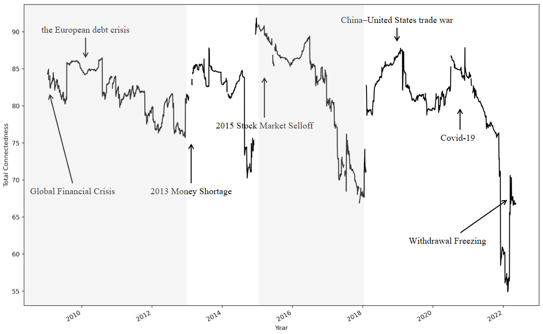
Figure 1: Rolling total connectedness.
Note: The rolling estimation window width is 300 days, and the predictive horizon for the underlying variance decomposition is 12 days. The shadowing parts represent the first (2008-2013) and third big cycle (2015-2018), and non-shadowing parts represent the second(2013-2015) and last big cycle(2018-present).
Some notable features are presented in figure 1. First, we could see similar pattern during different crises: the connectedness rise in the beginning of a stage and fall at the end of it. This means that each event had strongly influenced the dynamics of the volatility spillover. During a crisis the whole system would become more interconnected, which help the spread of shock among banks.
However, there is two different features of the last period (2018-present). First, there exists two crises in the last period, caused by the China-US trade war and COVID-19 respectively. Hence, the volatility spillover experiences a “W” shaped fluctuations within the 80%–87% band.
Second, unlike cycles before 2018, the total connectedness during COVID-19 era did not fluctuate around the highest value for a long time, instead it went down at the mid of 2020 when it hit a peak (85%), a similar movement during China-United States War. This means that the impact of the pandemic on banking system is not sustainable as before. According to Zihui Yang, the shock from the pandemic on finance industry doesn't last long either [35]. One explanation is that in this crisis, the financial, real estate, information technology and daily consumption industries have significantly increased their risk output during the event, while the healthcare, utilities and industrial sectors have become the main risk takers. Then the risk was spread to banking system as banks are the main financial source of these sectors. However, due to China's complete industrial system and effective pandemic prevention measures, the pandemic was effectively controlled, and the stock market was stabilized in February 2020. Thus, the total connectedness went down.
4.2.2. Total Directional Connectedness of Banks with Different Ownership
This sub-section we will investigate the structural changes of directional connectedness of banks with different ownership, which will lead us to observe the difference in contributions of volatility shocks from banks with different ownership.
Figure 2-4 presents the time series of total directional connectedness ("from","to" and "net" degrees) separately for banks of each ownership. The plots for total directional Connectedness "from" others are presented in the upper panel, the plots for total directional connectedness "to" others are in the middle panel, and the plots for "net" total directional connectedness to others are in the lower panel.
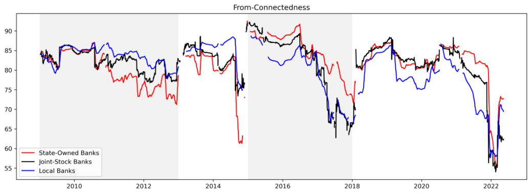
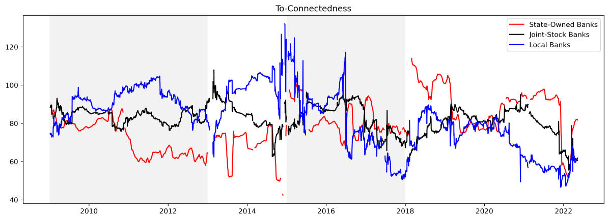
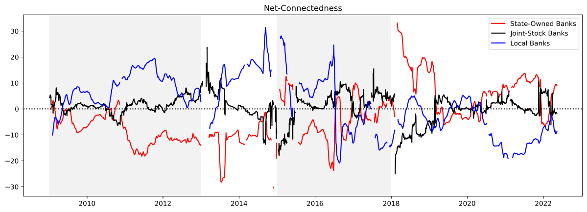
Figure 2-4: Total directional connectedness of banks with different ownership.
Note: Here we start with calculate the rolling estimation of directional connectedness of each bank.The rolling estimation window width is 300 days, and the predictive horizon for the underlying variance decomposition is 12 days.
First thing to notice is that the substantial difference between the "to" and "from" connectedness plots: The "from" connectedness of banks with different ownership is more similar than "to". This is not to hard to explain. Diebold stated that as banks are interconnected, the volatility shocks will be transmitted to each institution [2]. While the size of "to" shocks will be quite different due to the size and centrality of the banks, the total connectedness will be disturbed among other banks. That is why there is much less difference in the directional connectedness "from" others compared to the directional connectedness "to" others.
Then, as for the directional connectedness "from" others banks of different ownership, we could find it went through four notable cycles as the same as the total connectedness, moving within the 60%-90% range. The first cycle lasted from 2009 to 2012; the second from 2013 to 2014; the third from 2015 to 2017 and the last one from 2018 to 2021. This is not hard to be explained. Since the shock are always evenly disturbed among banking system as discussed in the section 4.1, the shape of the dynamic from-connectedness would be similar to the shape of the total connectedness (Figure 1).
Third, the directional connectedness from nationalized banks "to" others banks would rise when a crisis happens, while changes in connectedness across joint-stock banks and local banks do not exhibit a clear cyclical pattern. The reason is not hard to find. Since state-owned banks are systemically important banks in China with large bank size, we can expect this volatility shock to have a larger spillover effect on the stocks of other institutions whether the volatility shock is large or small [36]. As the nationalized banks have more international and complex business, the joint-stock banks and local banks are less influenced. As for joint-stock banks, their directional connectedness "to" other banks did not experience particularly drastic fluctuations (around 70% to 90%), probably because when we perform an arithmetic average on the connectedness of banks, the larger number of joint-stock banks reduces the volatility. For local banks, we can observe a decreasing trend in that last 10 years. This is mainly resulted from a decreasing connectedness from Ningbo Bank to other banks.
Last, since the time series of the total directional connectedness "from" other banks is relatively similar, the moving of the total directional connectedness "net" other banks is similar to that of the total directional connectedness "to" other banks.
One interesting finding here is that the "net" connectedness curves of local banks and state-owned banks are symmetric. And in the last period, there happened a structural change. To more precise, in the first three periods, nationalized banks are the receiver of the connectedness in the banking system, while local banks are the one spreading connectedness more than receiving it. In the last period, this pattern began to change with the state-owned banks sending more volatility shock to others than receiving it and local banks turning to receive shocks. This implies that state-owned banks became more contagious and the local banks became more vulnerable compared with their historical performance. As for joint-stock banks, the “net -connectedness” just fluctuate around 0 within the -20% to 20% band. This implies that the joint-stock banks' output and absorption are similar.
To sum up, we can see two main results in this sub-section. First, the movement of “from-connectedness” has clearer pattern than other two connectedness, and it always keeps the pace with the total connectedness. Second, in the last period, state-owned banks turn to risk emitters during a crisis from risk receivers, while the local banks turn to risk receivers from risk emitters. And the joint-stock banks' output and absorption are similar.
5. Conclusion
The main purpose of this research is to assess the volatility spillover effects caused by COVID-19, and compare it with the previous financial crises in the past 12 years in order to observe the heterogeneity effect of this pandemic. For this purpose, we apply the Diebold and Yilmaz volatility connectedness methodology to 14 important banks in China, including 4 state-owned banks [2], 7 joint-stock banks and 3 local banks. As their asset accounted for nearly 44% of the total assets of Chinese banking system, they could represent the Chinese banking system very well (as of Dec.31, 2021).
Our empirical results are as followings. Initially, we do find notable evidence about the important role of the COVID-19 played on the connectedness of Chinese banking system and its structure within the system. Statically, the findings show that the Chinese banks are highly interconnected especially during COVID-19 era. Indeed, the dynamic analysis expands this rule from COVID-19 era to other crises. Moreover, many big banks, during the pandemic, turned to send more volatility shock to the banking system, while small banks turned to a volatility receiver. This highlights the “too-big-to-fail” characteristic of Chinese banking system. Besides, we find a shock-passing path during the COVID-19 era, with big banks passing shocks to the middle banks, and the middle banks passing shocks to small banks. The reason behind this phenomenon is that when smaller banks are in crisis, they are more likely to borrow from bigger banks, which are more capable of resisting risk. However, as smaller banks have fewer assets than larger banks, they might be more likely to catch liquidity risk for not having enough capital to repay a loan.
With reference to heterogeneity features of ongoing crisis, we get two main findings. The first one is that the highly connected and contagious status of Chinese banking system didn't stay long during COVID-19 era, as we find that the total connectedness during the COVID-19 era did not stay high like previous crises, instead it dropped quickly as soon as it reached its peak. It is partly thanks to China's complete industrial system and effective pandemic prevention measures that the pandemic was effectively controlled, and the stock market was stabilized in February 2020. The second one is that during COVID-19 era, different from previous periods, state-owned banks began to send more volatility shock to others than receiving it and local banks turned to receive shocks, indicating that state-owned banks were more contagious and the local banks were more vulnerable compared with their historical performance.
Although there have been three years since the outbreak of COVID-19, and the WHO chief stated that “end of COVID pandemic is 'in sight'” in September 14, 2022, the study concerning with the impact of the COVID-19 on banking system and financial system has still long way to go. Future work could seek to identify the causes and implications of the heterogeneous features we find in this research, and assess the effectiveness of the policies regarding the post-crisis.
References
[1]. Barth, J.R., Li, L., Li, T., Song, F., 2013. Chapter 24 – Reforms of China's banking system. In: Beck, T., Claessens, S., Schmukler, S.L. (Eds.), The Evidence and Impact of Financial Globalization. Academic Press, San Diego, pp. 345–353.
[2]. Diebold F X, Yılmaz K. On the network topology of variance decompositions: Measuring the connectedness of financial firms[J]. Journal of econometrics, 2014, 182(1): 119-134.
[3]. Tobias A, Brunnermeier M K. CoVaR[J]. The American Economic Review, 2016, 106(7): 1705.
[4]. Zhou, C., 2010. Are banks too big to fail? Measuring systemic importance of financial institutions. Int. J. Central Bank. 6, 205–250.
[5]. Tarashev, N.A., Borio, C., Tsatsaronis, K., 2010. Attributing systemic risk to individual institutions. BIS Working Paper No. 308.
[6]. Acharya, V.V., Pedersen, L.H., Philippon, T., Richardson, M.P., 2017. Measuring systemic risk. Rev. Financ. Stud. 30, 2–47
[7]. Banulescu, G.-D., Dumitrescu, E.-I., 2015. Which are the SIFIs? A component expected shortfall approach to systemic risk. J. Bank. Finan. 50, 575–588.
[8]. Brownlees C, Engle R F. SRISK: A conditional capital shortfall measure of systemic risk[J]. The Review of Financial Studies, 2017, 30(1): 48-79
[9]. Billio M, Getmansky M, Lo A W, et al. Econometric measures of connectedness and systemic risk in the finance and insurance sectors[J]. Journal of financial economics, 2012, 104(3): 535-559.
[10]. Diebold F X, Yilmaz K. Better to give than to receive: Predictive directional measurement of volatility spillovers[J]. International Journal of forecasting, 2012, 28(1): 57-66.
[11]. Diebold F X, Yilmaz K. Measuring financial asset return and volatility spillovers, with application to global equity markets[J]. The Economic Journal, 2009, 119(534): 158-171.
[12]. Hautsch N, Schaumburg J, Schienle M. Financial network systemic risk contributions[J]. Review of Finance, 2015, 19(2): 685-738.
[13]. Wang G J, Xie C, He K, et al. Extreme risk spillover network: application to financial institutions[J]. Quantitative Finance, 2017, 17(9): 1417-1433.
[14]. Diebold F X, Liu L, Yilmaz K. Commodity connectedness[R]. National Bureau of Economic Research, 2017.
[15]. Wang G J, Xie C, Zhao L, et al. Volatility connectedness in the Chinese banking system: Do state-owned commercial banks contribute more?[J]. Journal of International Financial Markets, Institutions and Money, 2018, 57: 205-230.
[16]. Bubák, V., Kocˇenda, E., Zˇikeš, F., 2011. Volatility transmission in emerging European foreign exchange markets. J. Bank. Finan. 35, 2829–2841.
[17]. Antonakakis, N., 2012. Exchange return co-movements and volatility spillovers before and after the introduction of euro. J. Int. Financ. Markets, Inst. Money 22, 1091–1109.
[18]. Zhang, B., Wang, P., 2014. Return and volatility spillovers between China and world oil markets. Econ. Model. 42, 413–420
[19]. Maghyereh, A.I., Awartani, B., Bouri, E., 2016. The directional volatility connectedness between crude oil and equity markets: new evidence from implied volatility indexes. Energy Econ. 57, 78–93.
[20]. Antonakakis, N., Kizys, R., 2015. Dynamic spillovers between commodity and currency markets. Int. Rev. Financ. Anal. 41, 303–319
[21]. Liow, K.H., 2015. Volatility spillover dynamics and relationship across G7 fifinancial markets. North Am. J. Econ. Finan. 33, 328–365.
[22]. Apergis, N., Baruník, J., Lau, M.C.K., 2017. Good volatility, bad volatility: What drives the asymmetric connectedness of Australian electricity markets? Energy Econ. 66, 108–115.
[23]. Rizwan, M., Ahmad, G., Ashraf, D., 2020. Systemic risk: the impact of COVID-19. Finance Res. Lett. 36, 101682
[24]. Akhtaruzzaman, M., Boubaker, S., Sensoy, A., 2020. Financial contagion during COVID–19 crisis. Finance Res. Lett. 38, 101604
[25]. Amar, A.B., Belaid, F., Youssef, A.B., Chiao, B., Guesmi, K., 2021. The unprecedented reaction of equity and commodity markets to COVID-19. Finance Res. Lett. 38, 101853
[26]. Fasanya, I., Oyewole, O., Adekoya, O., Odei-Mensah, J., 2020. Dynamic spillovers and connectedness between COVID-19 pandemic and global foreign exchange markets. Econ. Res. Ekon. Istraz. 1–26
[27]. Matos, P., Costa, A., da Silva, C., 2021. COVID-19, stock market and sectoral contagion in US: a time-frequency analysis. Res. Int. Bus. Finance 57, 101400
[28]. Corbet, S., Goodell, J.W., Günay, S., 2020. Co-movements and spillovers of oil and renewable firms under extreme conditions: new evidence from negative WTI prices during COVID-19. Energy Econ 92, 104978
[29]. Garman M B, Klass M J. On the estimation of security price volatilities from historical data[J]. Journal of business, 1980: 67-78.
[30]. Demirer M, Diebold F X, Liu L, et al. Estimating global bank network connectedness[J]. Journal of Applied Econometrics, 2018, 33(1): 1-15.
[31]. Huang Q, De Haan J, Scholtens B. Analysing systemic risk in the Chinese banking system[J]. Pacific Economic Review, 2019, 24(2): 348-372.
[32]. Shen Y Y, Jiang Z Q, Ma J C, et al. Sector connectedness in the Chinese stock markets[J]. Empirical Economics, 2022, 62(2): 825-852.
[33]. Foglia M, Addi A, Angelini E. The Eurozone banking sector in the time of COVID-19: Measuring volatility connectedness[J]. Global Finance Journal, 2022, 51: 100677.
[34]. Jiang Z Q, Wang G J, Canabarro A, et al. Short term prediction of extreme returns based on the recurrence interval analysis[J]. Quantitative Finance, 2018, 18(3): 353-370.
[35]. Yang Zihui, Chen Yutian, Zhang Pingmiao. Macroeconomic Shock under Major Public Emergencies, Financial Risk Transmission and Governance Response [J]. Management World, 2020, 36(5): 13-35.(in Chinese)
[36]. Ouyang Zisheng, Mo Tingcheng. Research on Risk Spillover Effects of Systemically Important Banks Based on Generalized CoVaR Model [J]. Statistical Research, 2017, 34 (09): 36-43. DOI: 10.19343/j.cnki .11-1302/ c.2017 . 09.004. (in Chinese)
Cite this article
Li,J. (2023). Impacts of the COVID-19 Pandemic on Chinese Banking System: Measuring Volatility Connectedness. Advances in Economics, Management and Political Sciences,14,271-288.
Data availability
The datasets used and/or analyzed during the current study will be available from the authors upon reasonable request.
Disclaimer/Publisher's Note
The statements, opinions and data contained in all publications are solely those of the individual author(s) and contributor(s) and not of EWA Publishing and/or the editor(s). EWA Publishing and/or the editor(s) disclaim responsibility for any injury to people or property resulting from any ideas, methods, instructions or products referred to in the content.
About volume
Volume title: Proceedings of the 2nd International Conference on Business and Policy Studies
© 2024 by the author(s). Licensee EWA Publishing, Oxford, UK. This article is an open access article distributed under the terms and
conditions of the Creative Commons Attribution (CC BY) license. Authors who
publish this series agree to the following terms:
1. Authors retain copyright and grant the series right of first publication with the work simultaneously licensed under a Creative Commons
Attribution License that allows others to share the work with an acknowledgment of the work's authorship and initial publication in this
series.
2. Authors are able to enter into separate, additional contractual arrangements for the non-exclusive distribution of the series's published
version of the work (e.g., post it to an institutional repository or publish it in a book), with an acknowledgment of its initial
publication in this series.
3. Authors are permitted and encouraged to post their work online (e.g., in institutional repositories or on their website) prior to and
during the submission process, as it can lead to productive exchanges, as well as earlier and greater citation of published work (See
Open access policy for details).
References
[1]. Barth, J.R., Li, L., Li, T., Song, F., 2013. Chapter 24 – Reforms of China's banking system. In: Beck, T., Claessens, S., Schmukler, S.L. (Eds.), The Evidence and Impact of Financial Globalization. Academic Press, San Diego, pp. 345–353.
[2]. Diebold F X, Yılmaz K. On the network topology of variance decompositions: Measuring the connectedness of financial firms[J]. Journal of econometrics, 2014, 182(1): 119-134.
[3]. Tobias A, Brunnermeier M K. CoVaR[J]. The American Economic Review, 2016, 106(7): 1705.
[4]. Zhou, C., 2010. Are banks too big to fail? Measuring systemic importance of financial institutions. Int. J. Central Bank. 6, 205–250.
[5]. Tarashev, N.A., Borio, C., Tsatsaronis, K., 2010. Attributing systemic risk to individual institutions. BIS Working Paper No. 308.
[6]. Acharya, V.V., Pedersen, L.H., Philippon, T., Richardson, M.P., 2017. Measuring systemic risk. Rev. Financ. Stud. 30, 2–47
[7]. Banulescu, G.-D., Dumitrescu, E.-I., 2015. Which are the SIFIs? A component expected shortfall approach to systemic risk. J. Bank. Finan. 50, 575–588.
[8]. Brownlees C, Engle R F. SRISK: A conditional capital shortfall measure of systemic risk[J]. The Review of Financial Studies, 2017, 30(1): 48-79
[9]. Billio M, Getmansky M, Lo A W, et al. Econometric measures of connectedness and systemic risk in the finance and insurance sectors[J]. Journal of financial economics, 2012, 104(3): 535-559.
[10]. Diebold F X, Yilmaz K. Better to give than to receive: Predictive directional measurement of volatility spillovers[J]. International Journal of forecasting, 2012, 28(1): 57-66.
[11]. Diebold F X, Yilmaz K. Measuring financial asset return and volatility spillovers, with application to global equity markets[J]. The Economic Journal, 2009, 119(534): 158-171.
[12]. Hautsch N, Schaumburg J, Schienle M. Financial network systemic risk contributions[J]. Review of Finance, 2015, 19(2): 685-738.
[13]. Wang G J, Xie C, He K, et al. Extreme risk spillover network: application to financial institutions[J]. Quantitative Finance, 2017, 17(9): 1417-1433.
[14]. Diebold F X, Liu L, Yilmaz K. Commodity connectedness[R]. National Bureau of Economic Research, 2017.
[15]. Wang G J, Xie C, Zhao L, et al. Volatility connectedness in the Chinese banking system: Do state-owned commercial banks contribute more?[J]. Journal of International Financial Markets, Institutions and Money, 2018, 57: 205-230.
[16]. Bubák, V., Kocˇenda, E., Zˇikeš, F., 2011. Volatility transmission in emerging European foreign exchange markets. J. Bank. Finan. 35, 2829–2841.
[17]. Antonakakis, N., 2012. Exchange return co-movements and volatility spillovers before and after the introduction of euro. J. Int. Financ. Markets, Inst. Money 22, 1091–1109.
[18]. Zhang, B., Wang, P., 2014. Return and volatility spillovers between China and world oil markets. Econ. Model. 42, 413–420
[19]. Maghyereh, A.I., Awartani, B., Bouri, E., 2016. The directional volatility connectedness between crude oil and equity markets: new evidence from implied volatility indexes. Energy Econ. 57, 78–93.
[20]. Antonakakis, N., Kizys, R., 2015. Dynamic spillovers between commodity and currency markets. Int. Rev. Financ. Anal. 41, 303–319
[21]. Liow, K.H., 2015. Volatility spillover dynamics and relationship across G7 fifinancial markets. North Am. J. Econ. Finan. 33, 328–365.
[22]. Apergis, N., Baruník, J., Lau, M.C.K., 2017. Good volatility, bad volatility: What drives the asymmetric connectedness of Australian electricity markets? Energy Econ. 66, 108–115.
[23]. Rizwan, M., Ahmad, G., Ashraf, D., 2020. Systemic risk: the impact of COVID-19. Finance Res. Lett. 36, 101682
[24]. Akhtaruzzaman, M., Boubaker, S., Sensoy, A., 2020. Financial contagion during COVID–19 crisis. Finance Res. Lett. 38, 101604
[25]. Amar, A.B., Belaid, F., Youssef, A.B., Chiao, B., Guesmi, K., 2021. The unprecedented reaction of equity and commodity markets to COVID-19. Finance Res. Lett. 38, 101853
[26]. Fasanya, I., Oyewole, O., Adekoya, O., Odei-Mensah, J., 2020. Dynamic spillovers and connectedness between COVID-19 pandemic and global foreign exchange markets. Econ. Res. Ekon. Istraz. 1–26
[27]. Matos, P., Costa, A., da Silva, C., 2021. COVID-19, stock market and sectoral contagion in US: a time-frequency analysis. Res. Int. Bus. Finance 57, 101400
[28]. Corbet, S., Goodell, J.W., Günay, S., 2020. Co-movements and spillovers of oil and renewable firms under extreme conditions: new evidence from negative WTI prices during COVID-19. Energy Econ 92, 104978
[29]. Garman M B, Klass M J. On the estimation of security price volatilities from historical data[J]. Journal of business, 1980: 67-78.
[30]. Demirer M, Diebold F X, Liu L, et al. Estimating global bank network connectedness[J]. Journal of Applied Econometrics, 2018, 33(1): 1-15.
[31]. Huang Q, De Haan J, Scholtens B. Analysing systemic risk in the Chinese banking system[J]. Pacific Economic Review, 2019, 24(2): 348-372.
[32]. Shen Y Y, Jiang Z Q, Ma J C, et al. Sector connectedness in the Chinese stock markets[J]. Empirical Economics, 2022, 62(2): 825-852.
[33]. Foglia M, Addi A, Angelini E. The Eurozone banking sector in the time of COVID-19: Measuring volatility connectedness[J]. Global Finance Journal, 2022, 51: 100677.
[34]. Jiang Z Q, Wang G J, Canabarro A, et al. Short term prediction of extreme returns based on the recurrence interval analysis[J]. Quantitative Finance, 2018, 18(3): 353-370.
[35]. Yang Zihui, Chen Yutian, Zhang Pingmiao. Macroeconomic Shock under Major Public Emergencies, Financial Risk Transmission and Governance Response [J]. Management World, 2020, 36(5): 13-35.(in Chinese)
[36]. Ouyang Zisheng, Mo Tingcheng. Research on Risk Spillover Effects of Systemically Important Banks Based on Generalized CoVaR Model [J]. Statistical Research, 2017, 34 (09): 36-43. DOI: 10.19343/j.cnki .11-1302/ c.2017 . 09.004. (in Chinese)