1. Introduction

As a barometer of the market economy, the stock market not only indicates whether the socio-economic system is functioning well, but also affects the real income of stockholders [1]. If the stock market has been trending steadily upward, it can be concluded that the market economy is in a prosperous period, and stockholders can benefit from this prosperity of the market, and their shares are increasing in value. On the other hand, the market economy is likely in a period of recession or depression and stockholders face a greater risk of losing their investments if the stock market is in a startling or declining trend. Therefore, if investors can correctly forecast the trend of stock fluctuations, they can buy stocks at the bottom of the cycle and sell them at the top to gain benefits. The CSI 300 index is a "barometer" reflecting the complete functioning of the stock market and was chosen as the sample data for this study because it is the first index to describe the entire image of the Shanghai and Shenzhen stock markets since the formation of China's securities market [2].

The two most popular analytical techniques employed by academics to forecast stock values are time series models and linear regression models. Although the linear regression model is a widely used statistical tool for explaining one or more dependent variables using a collection of independent variables, it has substantial drawbacks [3]. According to Junhao Li, linear regression models can be used to anticipate when the stock market is steady, but they are unable to forecast the proper trend during times of turbulence and oscillation [4]. Complex time series models, which feature traits like volatility and non-stationarity compared to simpler linear regression models, can make up for the drawback that linear regression models cannot anticipate in oscillating markets [5]. With the exception of the medical sector, other sectors of the stock index have experienced a significant amount of shock over the past few years as a result of the COVID-19. And in accordance with the characteristics of the time series model analysis, this paper uses a time series model for forecasting.

In order to make short-term forecasts of the performance of stocks in various nations and sectors, researchers have built ARIMA models in a variety of scenarios. In the academic community, there have been many successful cases thus far. Yingchao Zhang and Yingjun Sun selected the closing price of SSE index from February 1, 2016 to October 16, 2018 as the research data to construct an ARIMA model to analyze and forecast the SSE index, which successfully confirmed that time series analysis can predict the trend of stock price fluctuations for a brief amount of time [6]. Ariyo A A, Adewumi A O and Ayo C K correctly predicted the stock price fluctuations of Nokia and Zenith Bank using the ARIMA model [7]. Mondal P, Shit L and Goswami S constructing ARIMA models to successfully predict the short-term movements of fifty-six stocks in different sectors in India [8]. Almasarweh M and Alwadi S confirm the ARIMA model's ability to anticipate the trend of banking stocks over the short term using a large amount of data [9].

2. Methodology

In the early 1970s, statisticians Box and Jenkins proposed the ARIMA method, which has the ability to precisely predict non-stationary time series. Time series' dynamic, continuous properties are examined by ARIMA models, which also show how the past, present, and future of time series are related [10]. The difference autoregressive moving average model is another name of ARIMA model. There are three parts in the model, the moving average process (MA), autoregressive process (AR), autoregressive moving average process (ARMA). According to the different situations, like whether the initial sequence is stable, researchers can take different process to establish model. And ARIMA model transforms non-stationary time series into stationary time series and regresses only the lag value of dependent variable and the present value of random error factor.

2.1. Data

The data's time window selected for the first time in this paper is from May 2017 to April 2022. The CSI 300 index closed every day except holidays is taken as the sample data of this study, with a total of 1217 valid data, as well as the daily yield of the CSI 300 index during this period. All data in this paper are from GuoTaiAn database. During the research process, it was discovered during the research process that the closing price of the CSI 300 index under this time period was not suitable for building an ARIMA model, and the specific causes will be discussed later. Then, the daily return of the CSI 300 index was used to build an ARIMA model to predict the fluctuation trend of that index's daily return in May 2022, which was then converted into closing price. The yield and share price are defined in the formula (1) and (2), as follows.

\( Yield = (share price of current period - share price of previous period) / share price of previous period \) (1)

Share price of current period = yield * share price of previous period + share price of previous period(2)

2.2. Model

BOX and Jenkins used 3 simple and practical steps to build the ARIMA model, namely (1) Identification (2) Estimation (3) Diagnostic checking. Obviously, this is only a simple step and it is still necessary to decide how to build the model on a case-by-case basis. So, the ARIMA model is constructed in five steps as follows.

(1) The smoothness of the series was identified based on the line graph, autocorrelation function and partial autocorrelation function of the time series, and the variance was tested by ADF unit root.

(2) The non-stationary series should be rounded. The data must be differentiated if the data series is non-stationary and has an increasing or declining trend.

(3) Through the above steps, choose the appropriate model from AR, MA and ARMA models; the requirements of AR model are PACF p-order post-truncated and ACF trailing; MA model is PACF trailing and q-order post-truncated; ARMA model is PACF first p-bar irregular, followed by trailing, ACF first q-bar irregular, followed by trailing.

(4) After the model is selected, the time series model estimation is started, where the p-value corresponding to the selected model is less than 5, and it can be concluded the effect of the variable on the dependent variable is significant at the 5% level of significance.

(5) Get the results after forecasting and compare with the actual situation. The specific formula is as follows:

\( {Y_{t}}={φ_{0}}+{φ_{2}}{Y_{t-1}}+{φ_{p}}{Y_{t-p}}+{ε_{t}}-{θ_{1}}{ε_{t-1}}-{θ_{2}}{ε_{t-2}}-…-{θ_{q}}{ε_{t-q}} \) (3)

In the above equation, the actual value is expressed in terms of \( {Y_{t}} \) and the random error is represented by \( {ε_{t}} \) at t. \( {φ_{i}} \) and \( {θ_{j}} \) are the coefficients, p and q are integers commonly called autoregressive and moving averages, respectively.

3. Results

3.1. Analysis on the Time Series Trend and Correlation of CSI 300 Index

As Figure 1 shown, it can be seen that the CSI 300 Index is showing a rising trend and then a downward trend from 2017 to 2018. In 2019, it shows a slow upward trend. 2020 shows an upward trend in the first half of the year, and the upward trend in the second half of the year is not as obvious as the first half of the year. 2021 shows a slow downward trend. Overall, from 2017 to 2022, the fluctuation of the CSI is amplitude and unstable.

Figure 1: The closing price of CSI 300 index from May 2017 to April 2022.

(Photo credit: Original)

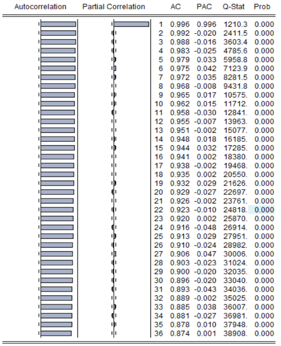
Figure 2: Autocorrelation and skewness analysis of CSI 300 index.

(Photo credit: Original)

Figure 2 shows the results of the autocorrelation and bias correlation analysis of the CSI 300 index. It is evident that by the 36th period, the ACF of the CSI 300 Index is still not eliminated, and by the 2^nd period PACF of the CSI 300 Index is eliminated. This situation does not fit any of the models stated in 2.2, indicating that the time series variable is unstable and needs to be differenced to eliminate the unstable phenomenon.

3.2. Differential

From Figure 3, it can be seen that the overall fluctuations of the CSI indices are leveling off after the first-order differential. It meets the requirements of constructing ARIMA model. In addition, Figure 5 demonstrates the result of autocorrelation and partial correlation analysis on the CSI after first-order differencing. it can be seen that the ACF of the first-order differential CSI is all eliminated and the trailing phenomenon of PACF is all absent, indicating that the time series variable is not suitable for ARIMA model.

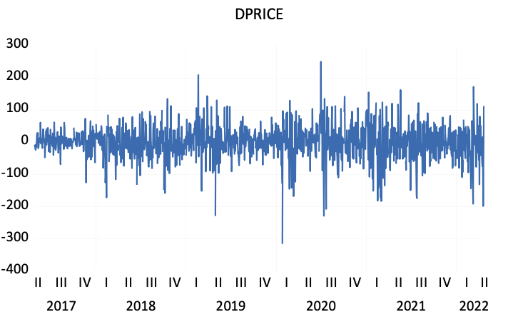
Figure 3: First-order differential stock price chart of CSI 300 index from May 2017 to April 2022.

(Photo credit: Original)

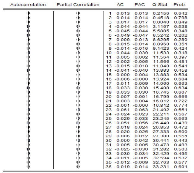
Figure 4: Autocorrelation and partial correlation analysis of the CSI after first-order differencing. (Photo credit: Original)

3.3. Constructing an ARIMA Model Using Returns and Forecasting

Obviously, the direct use of daily closing prices of CSI 300 index to construct ARIMA model will have a large error because its autocorrelation and partial autocorrelation tests cannot satisfy any of the three models, AR, MA, and ARMA. Therefore, this paper uses the relationship between yield and daily closing price, take the daily yield of the same period as the research data, and construct an ARIMA model to predict the data of May 2022, and then transform the yield into the closing price to achieve the final goal of predicting the closing price fluctuation. The specific calculation process is as previously mentioned Formula (1) and (2).

3.3.1. Time Series Trend Analysis and Testing on the CSI Index Returns

Figure 5 demonstrates that the overall volatility tends to be stable following the first order difference in the daily yield of the CSI 300 Index, which is necessary for the construction of the ARIMA model.

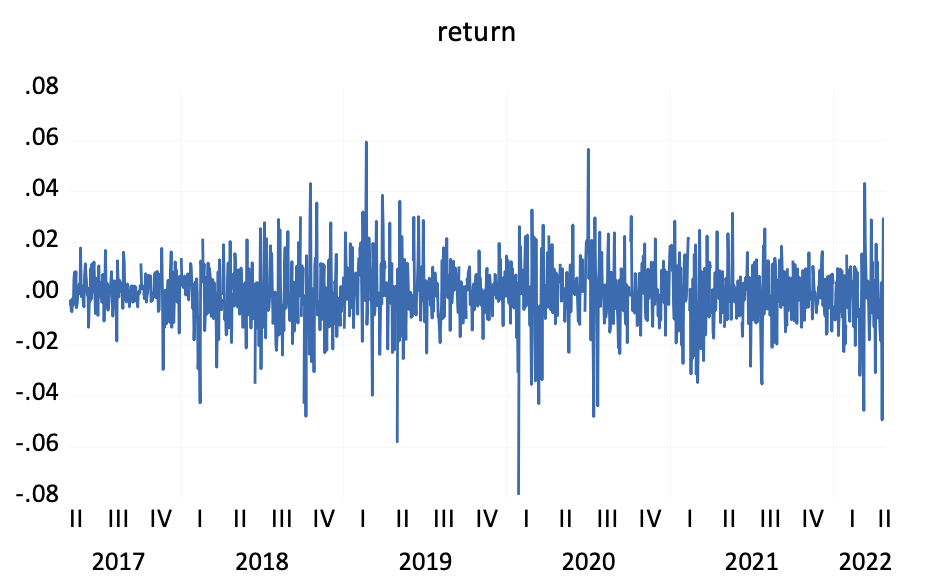
Figure 5: Time series trend of CSI returns.

(Photo credit: Original)

According to the Augmented Dickey-Fuller test statistic in Table 1, the t-value is -34.95884, and the associated p-value is below the significance threshold of 0.01, which means that the CSI index return rejects the original hypothesis "the variable is not smooth", indicating that the CSI index return fluctuates smoothly and the ARMA model can be constructed.

Table 1: Augmented Dickey-Fuller test statistic.

*MacKinnon (1996) one-sided p-values.

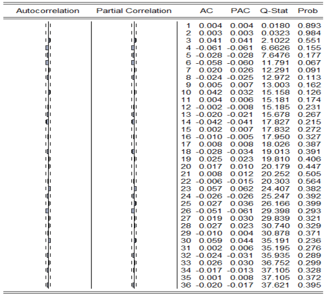
Figure 6: Autocorrelation and skew-correlation analysis of CSI index returns.

(Photo credit: Original)

Figure 6 shows the result of the autocorrelation and partial correlation analysis on the CSI index returns. It can be seen that the autocorrelation coefficient of the CSI index returns is at the 3rd order truncated tail and the partial autocorrelation coefficient is at the 3rd order truncated tail, which is in line with the requirements of constructing the ARMA model mentioned in the previous section, so it is initially decided to construct the model in ARMA (3,3).

3.3.2. Constructing ARMA Model

Table 2 shows the empirical results based on ARMA model, and Figure 7 indicates the testing results of autocorrelation and partial autocorrelation of the residual series. It can be learned that the residual series of the CSI index return equation is basically a smooth series with zero mean, and the autocorrelation coefficients and partial autocorrelation coefficients of the residual series of the CSI index return equation are not serially correlated, therefore, it can be predicted with the help of ARMA(3,3) model.

Table 2: ARMA model.

Figure 7: Correlation plots of the residual series of the CSI index return equations.

(Photo credit: Original)

3.3.3. Forecasting Results

Figure 8 shows the comparison between the predicted results and the actual data. As it can be clearly see in the graph, the blue line indicates the forecast index price and the yellow line indicates the real situation. Because of the long time span, the horizontal coordinate is one unit per 2 days for the coordinate scale. The blue and yellow lines in the entire table, the initial period from May 5, 2022 to May 11, 2022, the real situation by the holiday effect than the forecast situation price index is low, the specific reasons will be explained in detail in later chapters. But then the yellow curve quickly returned to 4000 points, always maintaining the 4000 points fluctuations, and the two lines are very close to each other. From the trend of the two lines in this graph, the situation predicted by ARIMA in this paper is very close to the real data, which is a strong evidence to prove that ARIMA has short-term forecasting ability.

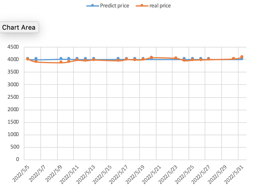
Figure 8: Comparison of forecast results and actual trend forecast.

(Photo credit: Original)

4. Discussion

The current sample data includes the extreme data of these years affected by the COVID-19, for example, the world was hit by the epidemic, in which the stock markets of several countries, including the United States, Canada, Brazil and South Korea, experienced multiple meltdowns. Within two weeks in March 2020, the U.S. stock market suffered four meltdowns within this short period of ten days, and the U.S. stock market collapsed in response. The Chinese stock market was also greatly affected, with all industry sectors except the medical sector beginning a prolonged downturn and severe fluctuations in stock market values. if the prediction can still meet the expected results under the influence of such external factors, it can prove that the time series model can make correct predictions than the linear regression model under the volatile and oscillating market; secondly, at the beginning of May 2022, the real CSI 300 index closing price appeared to be down, while the predicted index is more stable. This phenomenon can be explained by the holiday effect: either international or domestic holidays will have a negative impact on stock market returns [11]. This is a typical phenomenon in famous Chinese festivals, including the Spring Festival, Mid-Autumn Festival, National Day, and May Day. The stock prices around these holidays are volatile and cannot be predicted precisely. This is also an obvious drawback of this article, which cannot take into account too many complex situations, including unexpected public events and the inner thoughts of investors.

5. Conclusion

From the above graph, it is easy to conclude that the predicted and actual index prices obtained satisfactory results in terms of fluctuation trends and specific values, except for the holiday effect received at the beginning of the month. This paper puts forward the goal of establishing ARIMA model to predict the price of CSI 300 index. And the outcomes of the experiments using the ARIMA model show that the model has the ability to forecast short-term changes in stock values by using long-term time sample data. In this way, the construction of the ARIMA model can assist stock market investors in making wise investment choices. Also, research scholars can compare the data obtained from ARIMA simulations with the displayed data, and when large differences occur between the two, further research can be conducted to gain insight into what complex reasons are affecting the price of the stock. According to the results obtained, the ARIMA model can be more competitive than the linear regression model in terms of short-term forecasting. At the same time, this paper has some limitations. Forecasting fluctuations in stock price indices cannot fully take into account the effects of artificial factors such as holiday effects.

References

[1]. Xianzhong Tian, Anna Hu, Siyi Gu. A time series chain-based stock market forecasting method [J]. Journal of Zhejiang University of Technology,2021,49(5):503-510,563.
[2]. Wang, Nong-Shi. Simulation study on volatility of CSI 300 index based on GARCH family model [J]. China Business Journal,2022(1):100-102.
[3]. Li Y. Multiple linear regression model and stock sector index prediction [J]. National Circulation Economy,2017(10):62-63.
[4]. Li, J. H.. An improved multiple linear regression based stock price forecasting model [J]. Science and Technology Economic Market,2019(8):61-62,64.
[5]. Wang Xiaohong,Wang Mengyao,Hao Ting. Research on improved time-correlated serial stock price hybrid forecasting model [J]. Science and Technology for Development,2020,16(6):672-678.
[6]. Zhang Yingchao,Sun Yingjun. An empirical study on the analysis and forecasting of SSE index based on ARIMA model [J]. Journal of Economic Research,2019(11):131-135.
[7]. Ariyo A A, Adewumi A O, Ayo C K. Stock price prediction using the ARIMA model [C]//2014 UKSim-AMSS 16th international conference on computer modelling and simulation. IEEE, 2014: 106-112.
[8]. Mondal P, Shit L, Goswami S. Study of effectiveness of time series modeling (ARIMA) in forecasting stock prices[J]. International Journal of Computer Science, Engineering and Applications, 2014, 4(2): 13.
[9]. Almasarweh M, Alwadi S. ARIMA model in predicting banking stock market data [J]. Modern Applied Science, 2018, 12(11): 309.
[10]. Wang Yiting,Wei Jiangying. An empirical study of SSE 50 full return quotes based on ARIMA model [J]. Global Market,2018(16):55,57.
[11]. Jiang Yitao,Yang Linyan. A study on the holiday effect of Chinese stock market [J]. Economic Economics,2009(6):135-138.
Cite this article
Hou,J. (2023). Stock Index Prediction Based on ARIMA Model. Advances in Economics, Management and Political Sciences,14,319-328.
Data availability
The datasets used and/or analyzed during the current study will be available from the authors upon reasonable request.
Disclaimer/Publisher's Note
The statements, opinions and data contained in all publications are solely those of the individual author(s) and contributor(s) and not of EWA Publishing and/or the editor(s). EWA Publishing and/or the editor(s) disclaim responsibility for any injury to people or property resulting from any ideas, methods, instructions or products referred to in the content.
About volume
Volume title: Proceedings of the 2nd International Conference on Business and Policy Studies
© 2024 by the author(s). Licensee EWA Publishing, Oxford, UK. This article is an open access article distributed under the terms and
conditions of the Creative Commons Attribution (CC BY) license. Authors who
publish this series agree to the following terms:
1. Authors retain copyright and grant the series right of first publication with the work simultaneously licensed under a Creative Commons
Attribution License that allows others to share the work with an acknowledgment of the work's authorship and initial publication in this
series.
2. Authors are able to enter into separate, additional contractual arrangements for the non-exclusive distribution of the series's published
version of the work (e.g., post it to an institutional repository or publish it in a book), with an acknowledgment of its initial
publication in this series.
3. Authors are permitted and encouraged to post their work online (e.g., in institutional repositories or on their website) prior to and
during the submission process, as it can lead to productive exchanges, as well as earlier and greater citation of published work (See
Open access policy for details).