1. Strategy Overview

Compare different nations' purchasing power by using purchasing power parity and do valuations based on that data. What we believe is that PPP will help us to know the fair value of a currency. Since PPP can also be seen as a tool that reflects a nation's economic condition, such as whether it is in inflation or not, the best way to view purchasing power is to consider it a medium of the exchange rate. The Big Mac Index would be a typical example, like the exchange rate between RMB and USD does not consider personal income, but with the Big Mac Index, you can see the living condition of these two nations. Based on the valuation, long undervalued currencies and short overvalued currencies are determined.

In this strategy, investors will use the current exchange rate of a particular currency divided by its PPP value to generate a valuation of this specific currency. PPP value is the spot exchange rate of the same good in different countries. If the valuation is higher than 1, the currency is overvalued since the outside-shown value of the good proceeds its inner real value, and vice versa. In addition, if the currencies in the universe all have valuations that are lower (or higher) than 1, it is essential for investors to either only enter the trade on one side or still do hedging with high returns and high losses.

This strategy rebalances the portfolio quarterly. Firstly, Investors will long the top 30% currencies with the highest valuation calculated based on absolute PPP and short the bottom 30% currencies with the lowest valuation calculated by absolute PPP. Secondly, investors will use equal weighting to allocate capital for the chosen currencies. For example, they are using 50 million too long and 50 million too short. Finally, investors will rebalance after three months based on last quarter's data.

We estimate that PPP has a low annualized return, about 7.82%. Small Sharpe ratio, about 0.36. and low volatility, about 9.33%. Maximum drawdown has dropped a lot, down -26.40%. The PPP strategy risks if the price and exchange rate are not adjusted according to the PPP.

2. Specification

2.1. Analysis

PPP strategy is about comparing different nations' purchasing power by using purchasing power parity and doing valuations based on that data. What we believe is that PPP will help us to know the fair value of a currency. Since PPP can also be seen as a tool that reflects more accurately on a nation's economic condition, such as whether it is in inflation or not, and the best way to view purchasing power is to consider it as a medium of the exchange rate with more factors taken into consideration. The Big Mac Index would be a typical example, like the exchange rate between RMB and USD does not consider personal income. However, with the Big Mac Index, you can see the living condition of these two nations. Based on the valuation, we can see undervalued currencies and overvalued currencies. Later, we will trade based on these signs of currencies, be more specific, long undervalued ones and short those overvalued ones. Since PPP can be seen as a medium that reflects current trends and exchange rates more accurately, so this is why we believe in such an evaluation.

Besides using the Sharpe ratio, volatility, return, and max drawdown, some other indexes we would like to add are the kurtosis of return and Calmar ratio; a more detailed description of return is given in this index. Secondly, the Calmar ratio can also be a great tool that calculates the risk of a particular strategy, which is known for being up-to-date.

3. Data

3.1. Universe

Our universe will be G10 currencies and the Chinese Yuan. This is because we believe they are the most liquid and popular traded currencies globally, and it is the most representative market for us to trade. Also, linking the G10 currencies with the Chinese Yuan allows us to understand better the fair value of the goods in different countries.

3.2. Data Sets

Since most of our group lives in China, it is easier to get a sense of the approximate value of the good in China, which means it is easier to compare those values with G10 currencies. Our Data Sets will be the exchange rate between the G10 currencies compared to the Chinese Yuan. Moreover, there will be a total of 10 data sets. Also, we will collect the PPP value of these currencies, along with their short-term interest rate

3.3. Data Sources

The Exchange Rate comes from Yahoo Finance [1,2], and both the PPP value and short-term interest rate are from OECD [3, 4].

3.4. Data Range

We would set our data range from January 1st of, 2010 to December 31st of 2021. Our In Sample range will be from 2010 to 2018, ensuring that we can effectively adjust our strategy after running the backtests of the more recent years with the pandemic. We set the Out of Sample range as 2019-2021.

4. Strategy Detail

4.1. Signal Generation

PPPs are long-term and complex arrangements that require a thorough understanding of duties and responsibilities and risk-sharing between the parties. Compare different nations' purchasing power by using purchasing power parity and do valuations based on that data [1]. What we believe is that PPP will help us to know the fair value of a currency. Since PPP can also be seen as a tool that reflects a nation's economic condition, such as whether it is in inflation or not, the best way to view purchasing power is to consider it a medium of the exchange rate. Based on the valuation, long undervalued currencies and short overvalued currencies are determined. First of all, there are two types of PPP. The first one is Absolute PPP (APPP) which ignores inflation, challenging to implement in the real world. The formula is:

APPP= Cost of good X(currency one)/cost of good X(currency two)(1)

The second one is Relative PPP (RPPP) which is adjusted for inflation. The formula is:

S(adjusted)=APPP[(1+inflation A)/(1+inflation B)](2)

The valuation formula is:

(Average exchange rate over three months)/ Relative PPP.(3)

Typically currencies in the long portfolio need to have a valuation lower than 1, and the currency in the short portfolio should be higher than 1. Our universe will be G10 currencies, and our base currency is the Chinese yuan. For example, EUR exchange rate is 0.15, so the PPP is 21/23, equal to 0.91 for good(X). This valuation is 0.16, much smaller than 1, so we should take this in an extended portfolio. Also, take JPY as another example; the exchange rate is 19.96, so the PPP is 30/10, equal to 3, and the valuation is 6.65, which is also bigger than 1, so we should short this currency. Rank the results short, the Top 3, and the bottom 3.

4.2. Portfolio Construction

4.2.1. Trading Frequency

This strategy rebalances the portfolio monthly.

4.2.2. Selection (Hedging)

We have two options: enter a trade on only one side, or go long. Alternatively, we can still go long bottom three and short top 3. In this case, the short portfolio will yield negative returns, while the long portfolio will yield more favorable returns. Firstly, Investors will long the top 30% currencies with the lowest valuation calculated based on relative PPP and short the bottom 30% currencies with the highest valuation calculated by relative PPP.

4.2.3. Sizing

Investors will use equal weighting to allocate capital for the chosen currencies. After a month, investors will rebalance based on the last monthly data. An equal-weighted index is a stock market index that gives equal value to all the included stocks. In other words, each stock in the index has the same importance when determining the index's value, regardless of whether the company is large or small or how many shares are trading for. So in this strategy, we will allocate each currency of long and short by 33.33%

4.2.4. Trade Execution

During the execution, investors should consider several possible transaction costs. Transaction cost is calculated by the following formulas. Pip is also called “percentage in point” (usually =0.0001), a unit of spread. Pip value =

(1 pip / current exchange rate) * trade amount, transaction cost = pip value * spread in pips

In this case, the bid and ask cost is about 40000 dollars. Besides, swap rate cost and legality should also be mentioned in this strategy. Swap rate cost=

difference between the overnight interest rate for two currencies that a Forex trader is holding

The stabilities and government policies of issuing countries would lead to risks, such as the government's regulated RMB, so some trades are limited. In order to minimize transaction costs, investors could trade at regular trading sessions and avoid spreads by paying commissions to the platform. It usually costs 1% to 2% of the investments; in this case, it costs 10000 dollars. Hence, the entire transaction cost of this strategy is around 50000 dollars.

4.3. Implementation

The cumulative PnL graph shows a continuous fluctuation and an overall trend of gaining profit. Starting from 2010/01/01, the strategy's profit grew slowly. After 2013/01/30, the curve got a higher slope and peaked at 417701.80 on 2015/11/17. Then, the curve turned the direction and started losing money from the end of 2015 to approximately September 2017. Moreover, the curve then started going up slowly and finally reached 342912.88 as the result of the strategy. In the PnL graph, we took short-term interest rate into account and modified our net value formula as follows:

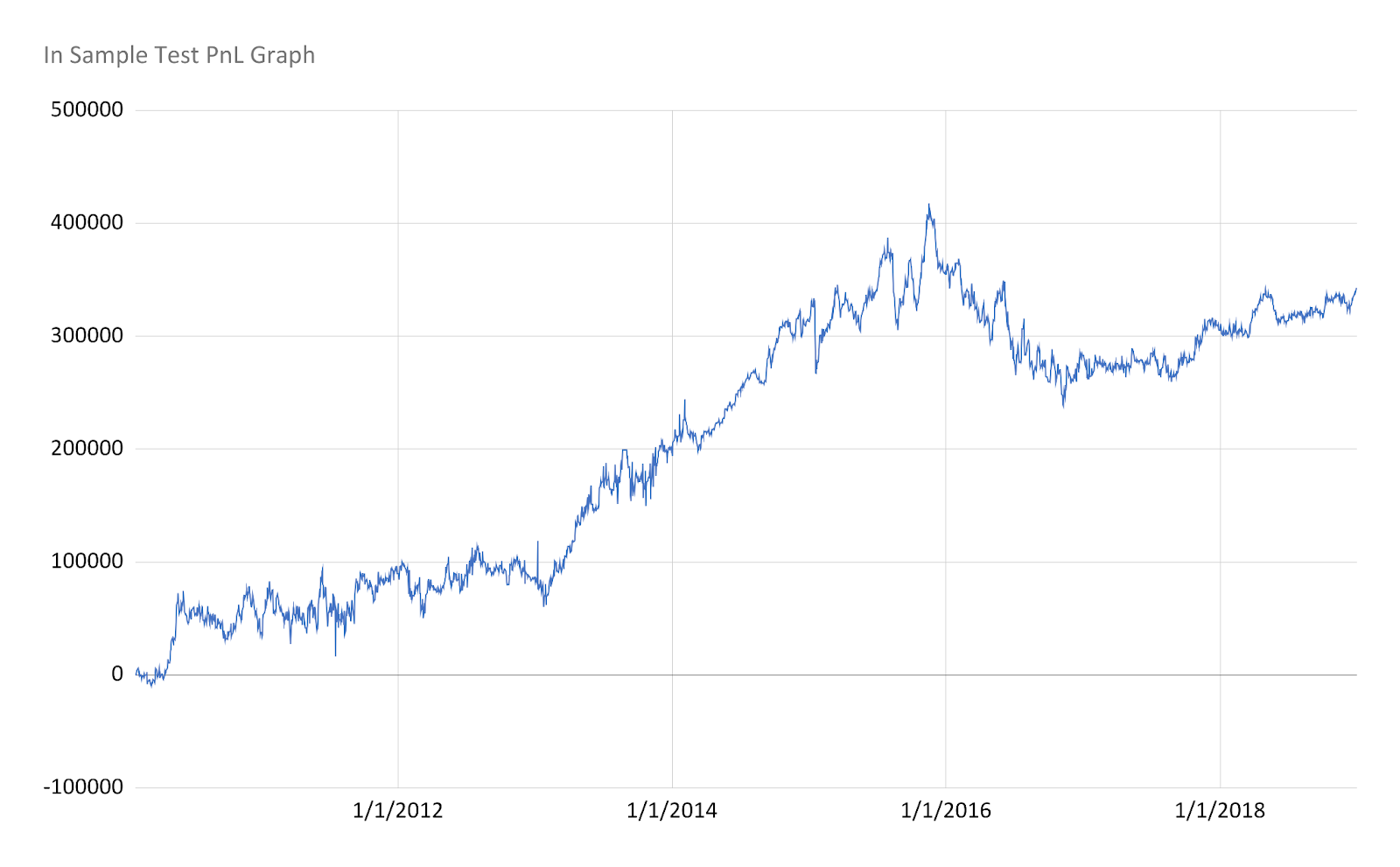
Figure 1: PnL graph.

Day 2 Net Value=Day 1 Net Value*(1+'Exchange Rate(Day 1))*Short-Term Interest Rate

The currencies in the long portfolio usually have a much greater interest rate than those in the short portfolio. So, in this case, we gain more profit when we hold these currencies with high interest rates. Moreover, this results in a 34% final profit.

Table 1: The sharpe ratio for this strategy is 0.417258.

Sharpe Ratio

The Sharpe Ratio for this strategy is 0.417258. Based on the formula of Sharpe Ratio:

It has annualized Return/Annualized STD of Return. It can be seen that the return rate is much lower than its standard deviation. This means that the strategy has a high risk. The variation of return is far beyond the return rate, and the risk that the strategy encounters is not offset well enough by its return; in other words, the strategy does not offer enough excess return considering its volatility. In this case, it is reasonable to have a 1.81% annualized return with a volatility of 0.046.

4.4. Kurtosis and Calmar Ratio

In order to further measure this strategy, I also measured the kurtosis of return and the calmar ratio of this strategy. I first measured the kurtosis with annualized data, and it turned out to be extremely low on daily return percentage was 0.282537. Indicates that during the in-sample backtest, PPP performed a stable return, and only a few cases of extreme return occurred. Secondly, after annualizing the return rate, the Calmar ratio was also in a relatively low range of -0.0015608, which tells us that PPP has a shallow risk. Both indexes have shown that the PPP strategy has performed a stable return range and low risk.

4.5. Risk

The in-sample risk is about 41.9566. In this case, the beginning is to calculate daily % return and volatility (variance and SD). Then annualize daily % return. In the process of annualization, every timeline 333333.3333 is encountered, and the blank of the previous daily return is deleted, which leads to the error of daily % return. Every month from 2010 to 2018 needs to be cleaned up. So, I integrated the annualized values for each month separately. The result of it is also more extensive enough since the return fluctuates wildly.

4.6. Volatility

The in-sample annualized volatility is 0.04281324816, about 4.28%. The calculation is made using the formula volatility over a time horizon =

the standard deviation of returns * square root of the number of periods in a time horizon

It can be seen that volatility has been low for nine years. Prices also fluctuate as currencies affect many factors, including political, economic, and social events. Since the monthly returns are pretty small, the volatility is low.

4.7. Transaction Cost

This strategy's in-sample swap cost is 6919.71, and the out-of-sample swap rate cost is 2791.53. According to the formula: Swap interest ﹦

An actual number of orders placed × standard of 1 lot × exchange rate price (short and long prices are different) × interest accrual days × annual interest rate difference / 360 days this cost is relatively small compared with the cumulative return and has little impact on the final return. The overall transaction cost is 59711.24. Bid-ask spread cost is the biggest among the entire cost, which means that the price fluctuation caused by different trading hours is enormous. Therefore, high platform fees will be inevitable.

4.8. Differences From Expectation

In the IS, our expectation of volatility is about 9.33%, and our actual result was 4.67 percent. So, it was 3.15% lower than expected. The quick ratio in our expectation is 0.36, which is smaller than the actual result of 0.417258. The annualized return in the expectation is about 7.82%. The actual return is 1.81% which is lower than the expectation.

5. Conclusion

Similar to the In Sample backtest, the OOS also experienced high fluctuations from 2019 to 2021. With a negative trend, the graph shows a loss of 44,115.60 at the end of the backtest period. However, unlike the IS PnL graph, the OOS graph shows a limited period–only from January to approximately August 2019 and March to May 2020–when the strategy gains significant profit. This is because the interest rates of the long portfolio are significantly lower than the IS period, in this case, the strategy loses money due to high inflations in recent years.

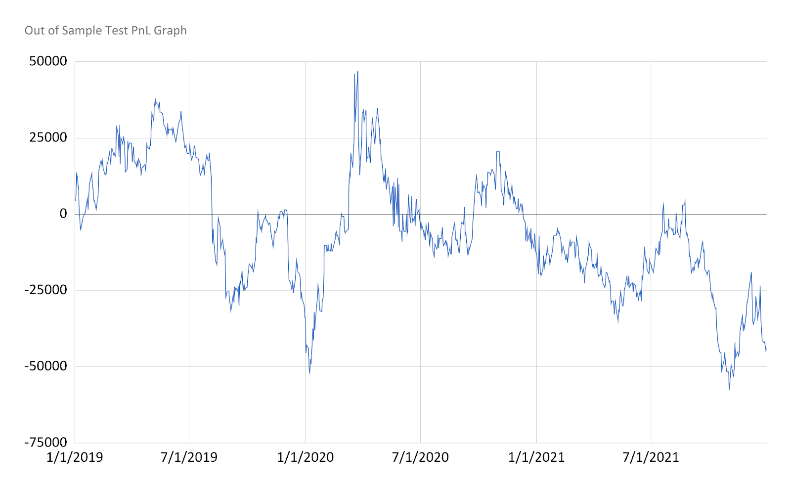
Figure 2: Out of sample PnL graph.

Table 2: The sharpe ratio for the OOS backtest is -0.19961.

Sharpe Ratio

The Sharpe Ratio for the OOS backtest is -0.19961; this negative value is due to the negative return. In this case, in addition to the high risk, the predicted return for this portfolio is not appreciated. Overall, the Sharpe ratios from both IS and OOS provide convincing evidence that the strategy could generate little or even negative returns with inevitable volatility, so it is essential to improve this portfolio and formulas to generate an acceptable positive return and Sharpe ratio for recent years.

5.1. Kurtosis and Calmar Ratio

During the out-of-sample period, the calmar ratio was 0.003715, which remained a relatively constant number as the in-sample backtest. Clearly illustrates that the PPP strategy is low risk. On the other hand, while kurtosis was 3.3019, it was pretty different from the in-sample part's calculation; there are few possible causes for that differentiation, it could be affected by a short period, and if we look at long term, kurtosis of PPP strategy is more likely to be flat and platykurtic; or there have been dynamic changes happened. Additionally, the negative Sharpe ratio in the oos test and high volatility provided evidence for the two downsides I mentioned.

5.2. Risk

The out-of-sample annualized risk is 45.7857. However, it turns out that when I continued to do risk for 19 to 21 years, I directly calculated variance and SD for the value of daily % return, and these two values were quite large. The reason is that Daily returns fluctuate considerably.

5.3. Volatility

The out-of-sample annualized volatility is 0.03320377673, about 3.32%. This is calculated based on the standard deviation of returns in the last three years. It can be seen that the volatility is minimal in comparison. It can be seen that in recent years, the foreign exchange market has still been relatively stable.

5.4. Additional Considerations

First, this paper only uses ten years of data for sample calculation. We recommend extending the data range to 30 years for more precise analysis. In addition, we use absolute PPP, which ignores inflation; thus, this strategy can hardly be implemented in real life. Finally, when calculating transaction costs, we use almost the same group of currencies each year for simplification. Although swap rate cost seems to have little impact on the final return, we should consider daily changes to judge precisely.

During implementation, we opted for equal weighting, which has less risk but less reward by comparison. Moreover, the equal weighting will be simpler to implement. On the other hand, if our strategy adopts signal weighting, the return should be slightly higher. When selecting a currency for short, in the PPP strategy, we should select the overvalued currency, the currency with an absolute PPP greater than 1. However, since China is a developing country based on CNY, its purchasing power will be lower than that of g10. So, all absolute PPP values are less than 1. Therefore, we can only take the currency of the most significant three values for short, making it more likely to lose money on the short because they are all undervalued on a CNY basis.

5.5. Trading Recommendation

Our recommendation is not to trade this strategy. Through indexes like the information ratio, Calmar ratio, and Sharpe ratio, PPP has proved to be a stable strategy for such a duration. Even when losses occur, it does not come in huge numbers, again proving its stability, but it also reveals its disadvantage of creating huge returns. During the in-sample period, it has shown its disadvantage because once huge losses appear, PPP will fail to make that money back. Furthermore, a hidden risk is also caused by highly unchanged shorting and long lists during most trading dates.

References

[1]. CMC Markets. (2022) A guide to forex trading strategies. 5 Forex Trading Strategies with Examples | CMC Markets. (n.d.).https://www.cmcmarkets.com/en/learn-forex/forex-trading-strategies.
[2]. Yahoo Finance. Exchange Rate https://finance.yahoo.com.
[3]. The OECD (2022 ) Monthly Interest Rate short-term interest rates - OECD data. https://data.oecd.org/interest/short-term-interest-rates.htm.
[4]. The OECD. (2022) Inflation rates - short-term interest rates - OECD data. (n.d.) https://data.oecd.org/interest/short-term-interest-rates.htm.
Cite this article
Shen,H.;Zheng,X.;Yin,M.;Peng,X.;Liu,Z. (2023). Trading Strategy–Purchasing Power Parity. Advances in Economics, Management and Political Sciences,15,68-76.
Data availability
The datasets used and/or analyzed during the current study will be available from the authors upon reasonable request.
Disclaimer/Publisher's Note
The statements, opinions and data contained in all publications are solely those of the individual author(s) and contributor(s) and not of EWA Publishing and/or the editor(s). EWA Publishing and/or the editor(s) disclaim responsibility for any injury to people or property resulting from any ideas, methods, instructions or products referred to in the content.
About volume
Volume title: Proceedings of the 2nd International Conference on Business and Policy Studies
© 2024 by the author(s). Licensee EWA Publishing, Oxford, UK. This article is an open access article distributed under the terms and
conditions of the Creative Commons Attribution (CC BY) license. Authors who
publish this series agree to the following terms:
1. Authors retain copyright and grant the series right of first publication with the work simultaneously licensed under a Creative Commons
Attribution License that allows others to share the work with an acknowledgment of the work's authorship and initial publication in this
series.
2. Authors are able to enter into separate, additional contractual arrangements for the non-exclusive distribution of the series's published
version of the work (e.g., post it to an institutional repository or publish it in a book), with an acknowledgment of its initial
publication in this series.
3. Authors are permitted and encouraged to post their work online (e.g., in institutional repositories or on their website) prior to and
during the submission process, as it can lead to productive exchanges, as well as earlier and greater citation of published work (See
Open access policy for details).