1. Introduction

Since an exchange rate determines the value of different currencies in relation to each other, it serves as an important indicator of the trade's determination and capital flow dynamics, which is high-profile for hedging judgements, capital budgeting decisions, and the assessments of earnings for both investors and governments. It’s also a helpful source for extracting information about economic and financial situations across time since it incorporates a number of economic variables and determinants. Governments can use that for monetary policy formulation and sometimes the adjustment of central bank's interventions when aiming to reduce the internal and external harm caused by undesirable interference movements. Also, accurate prediction of foreign currency rates is essential for large multinational company units as it increases their total profitability [1]. Investors, likewise, need more accurate forecasts to enable their investment analysis and asset allocation decisions. With the plunge trend of the two currency’s exchange rates as the forecasting objective, this paper first discussed the univariate ARIMA model's performance, so as the multivariate regression model with ARIMA errors, i.e. four macroeconomic variables supposed influential to the change of exchange rate incorporated in the AR part of the ARIMA model, is introduced and evaluated. The exchange rate is very important for measuring the economic development strength of countries, and the change of exchange rate can reflect the change of capital among countries to a certain extent. Based on this, this paper attempts to forecast the change of exchange rate from the perspective of exchange rate, laying a theoretical and practical foundation for economic development and related theories.

Section 2 previous work related to this study is reviewed. In section 3 macroeconomic theories are introduced respectively to explain the chosen variables. The data and methods details are described in section four. In section 5 the constructed models, univariate and the regression model with ARIMA errors, are used to forecast the 8-month plunge event of the exchange rates. The performance of the model is also discussed in this section. The conclusion is in section six.

2. Literature Review

A couple of methods have been utilized in the forecasting of exchange rate in the literature. Among them, autoregressive integrated moving averages (ARIMA) is an extensively discussed method. Dunis and Huang, used an ARMA (4, 4) model to estimate the future dollar/euro exchange rate [2]. Some elasticity was insignificant at the 95% confidence level, so their estimation is not good enough [3]. ARIMA model, by comparison, is a widely used model in literature. AKINCILAR, TEMİZ and ŞAHİN compared the performance of ARIMA model in forecasting exchange rate with the other four models in the context of a given time interval in Turkey. They came to a conclusion that the ARIMA model is not the most appropriate model in the case [4].

In recent years, more hybrid models with combined linear and nonlinear models can seemingly be a more effective way to improve forecasting performance instead of ARIMA. Three Artificial Neural Network (ANN) based forecasting models were investigated and compared with the traditional ARIMA model by Joarder Kamruzzaman and Ruhul A Sarker for Australian Foreign Exchange to predict six different currencies against Australian dollar [5]. In another study stated by Muhammad AsadUllah, Muhammad Adnan Bashir and Abdur Rahman Aleemi (2022), the exchange rate of Euro against the US dollar during the COVID-19 was forecasted using three univariate models (including ARIMA model) and one multivariate model (NARDL, i.e. nonlinear autoregressive distributive lags model) and the latter method performs the best [6].

However, the utter success of these hybrid models does not always seem to be the case. In a study proposed by Babu and Reddy, the conclusion is contradicted with existing literature since ARIMA model does better than those complicated nonlinear models, e.g. Neural Network and Fuzzy neurons in predicting the exchange rate market in India [7]. Consequently, it's aware that the ARIMA can still predict a situation just as well as any other hybrid complex model by being optimized to perform better.

3. The Fluctuation of the USD/EURO Exchange Rate Driven by Macroeconomic Theories

The exchange rate is deeply influenced by macroeconomic variables. The above-mentioned failures and limited explanation power of ARIMA models in forecasting the exchange rate implied that the prediction would be undesirable without other variables being taken into consideration. According to the research proposed by Ghalayini, for a long time, the PPP (Purchasing Power Parity) and the UIP (Uncovered Interest rate Parity) theory dominated the exchange rate theories, the two main equilibrium theories of the exchange rate. However, Ghalayini pointed out the Business cycles and the Money Aggregates should also be integrated as important impacting factors in the modeling of the exchange rate time series [3]. Similar points of view are presented by Weisang and Awazu [8]. Correspondingly, the four macroeconomic covariates that enter the study below are introduced as follows.

3.1. Interest Rate Parity

Interest rate parity (IRP) is an elementary relationship between exchange rates and interest rates. The exchange rate is seen as the mechanism that balances the interest rates differential. That's the reason why IRP can be conversely used to forecast the exchange rate. The immediate interest rate is chosen as the related variable, which represents the daily cost of money, both for USD and EUR. The difference between US and European immediate interest rate is used as one covariate.

3.2. Purchasing Power Parity

The theory of Purchasing Power Parity says that exchange rates are reverting to their PPP values in the case of the foreign trade balance. PPP is of great importance when predicting the exchange rate between countries. Xu use aggregate price indices to test the fitness of PPPs and forecast the exchange rate [9].

3.3. Money Aggregates

Money aggregates is a measurement of the stock of money in circulation within a country, which suggests the country's supply and demand condition and thereby influences the relative price of two currencies.

3.4. Business Cycles

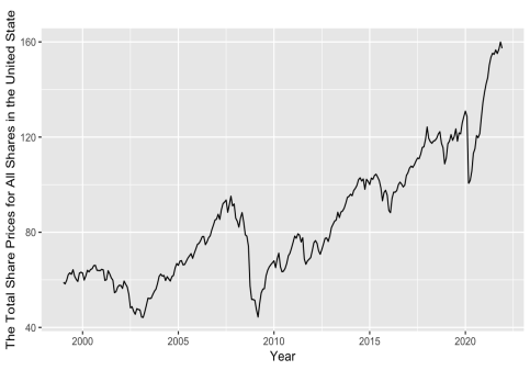
Business cycle can also be called as economic cycle. It refers to long-term economy-wide fluctuations in extensive economic activities when the economy is organized on free-enterprise principles. As a possible influential factor, the business cycle is tracked by share prices closely. To contain this ingredient, the total U.S. stock price is involved in the reference variables. The total share prices for all shares in the United States are presented.

Since 2022, high energy prices have contributed to rising CPI in the Eurozone, and the US is also suffering from high inflation. And the massive monetary easing in the US since COVID-19 has also led to the continuous rise of M2. The dollar's expectation of increasing interest rates is also pushing the gap between USD and EURO short-term interest rates to widen. Accordingly, the stock market, as a reflection of the economic cycle, also has uncertainty. In other words, the above four aspects as the impact factors of the USD/EURO exchange rate have experienced unusual changes since 2022.

In this paper, the attempt of modeling and predicting the USD/EURO exchange rate via ARIMA model is described, particularly, the capability enhancement of the model in forecasting the parity of the two currencies’ exchange rate is further discussed with the macroeconomic variables incorporated.

4. Methodology

4.1. Data

All data utilized in this paper is downloaded from FRED (https://fred.stlouisfed.org). In this study, the time series of monthly U.S. Dollars to Euro Spot Exchange Rate ("DEXUSEU ") is used to analyze and valid the forecasts [10].

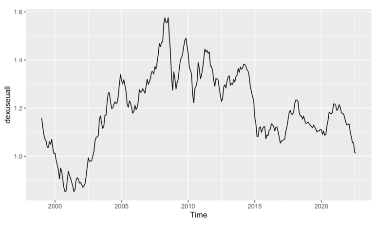
Figure 1: The monthly USD/EURO exchange rate from January 1999 to December 2021.

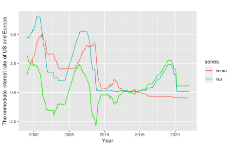
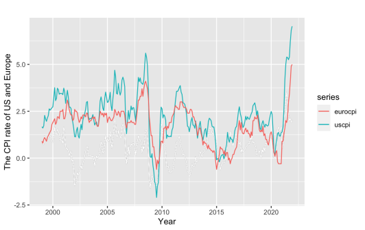
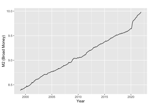
The macroeconomic-related variables, including Immediate Interest Rate for the US("IRSTCI01USM156N"), Immediate Interest Rate Total for the Euro Area (19 Countries) ("IRSTCI01EZM156N"), M2("WM2NS"), Total Share Prices for All Shares for the United States ("SPASTT01USM661N"), and Consumer Price Indices for US and Europe ("CPALTT01USM659N", "EA19CPALTT01GYM"), are taken as data sets starting from January 1999 and ending in December 2021 and are added to the more accurate ARIMA model based both on data and economic variables. All data series were checked. To unify the data and avoid the impact of vacant data on modeling and calculation, all data is downloaded monthly.

(a)

(b)

(c)

(d)

Figure 2: The monthly (a) immediate interest rate of USD and Euro, (b) US and Europe CPI index, (c) M2, and (d) total share prices for all shares for the United States (index 2015=100) during the period from January 1999 to December 2021.

The monthly time series of all variables cover the period from January 1999 to August 2022, among which, the period from January 1999 to December 2021 provides the training dataset to construct the ARIMA models, whereas the 8-month from January to August 2022 is the forecasted and validation period of the exchange rate.

4.2. ARIMA Modeling

ARIMA Model. ARIMA model is one of the popular approaches to time series forecasting. It was written in detail in most texts or documents about time series. The ARIMA model has been demonstrated effective to utilize the underlying correlation between the present and past lagged observations within a time series to forecast future results.

A non-seasonal ARIMA model is a combination of an Integrated (I) component (d), and ARMA model. The Integrated component represents the number of times the data needs to be differenced in order to reach stationary. ARMA, the second component, can be further decomposed into autoregression (AR) and moving average (MA) model constituent. The full model can be written as

\( {y \prime _{t}}=c+{ϕ_{1}}{y \prime _{t}}-1+…+{ϕ_{p}}{y \prime _{t}}-p+{θ_{1}}{ε_{t}}-1+…+{θ_{q}}{ε_{t}}-q+{ε_{t}} \) (1)

where \( y \prime t \) is the series have been differenced.

Generally, ARIMA has the form ARIMA(p,d,q), where p, q represents the order of the autoregressive part and the moving average part respectively, while d denotes the degree of differencing involved.

The modeling procedure with ARIMA is as follows:

First step is stationary Test (to determine d). The establishment of the ARIMA (p,d,q) model starts from the finite differencing applied to nonstationary data to make it stationary, i.e., statistical attributes like the mean and the autocorrelation variance are constant with time. In this step, the parameter d, the differencing times, will be obtained.

Second step is identification (to determine p and q). In this stage, a couple of potential the AR(p) or MA(q) models are selected by examining the plots of ACF and PACF against the lag lengths. Try the models and search for several candidate models by optimizing the Akaike information criteria (AIC) with smaller AICc values.

Third step is residuals Check. Perform fitted estimations using the tentative models and check the residuals by plotting the ACF and performing portmanteau tests. Once the residuals look like white noise, the model would be regarded as appropriate to estimate the time series and perform further forecasts. If not, the model should be redefined following the above steps.

Seasonal ARIMA Model. Seasonal ARIMA models can model a wide range of seasonal data. As an extension to ARIMA model, seasonal ARIMA model includes additional seasonal terms which is written as \( {ARIMA (p,d,q,) (P,D,Q)_{m}} \) , where \( { (P,D,Q)_{m}} \) represents the seasonal part of the model, and m = number of observations per year. When identifying the seasonality of the data USD/Euro Exchange Rate, the information in ACF and PACF plot is analyzed and their seasonal lags and significant spikes are found. In the part of presenting results, we consider the data seasonally and attempt to construct an appropriate seasonal ARIMA model to do a better forecast.

Regression with ARIMA errors. The ARIMA models can be extended to include explanatory variables in the models by allowing the errors from regression to contain autocorrelation. In R-Studio, the R function ARIMA() fits a regression model with ARIMA errors if the argument \( xreg \) , containing the vectors of all predictors \( x \) , is designated and used. In this study, \( xreg \) is designated by the four macroeconomic variables.

5. Results

5.1. Stationary Tests

The monthly time series and the one-order difference of the USD/EURO Spot Exchange Rate and the four macroeconomic variables are shown in Figure 3. Obviously, turning points can be identified at the beginning of 2020 for all variables (Figure 3a), which represent the macroeconomic impacts caused by the outbreak of the COVID-19. And from Figure 3b, their monthly changes (one-order differencing) oscillate around 0 and in fact, all of the differenced time series have passed the unit root tests, indicating all variables can be regarded as stationary with one-order difference.

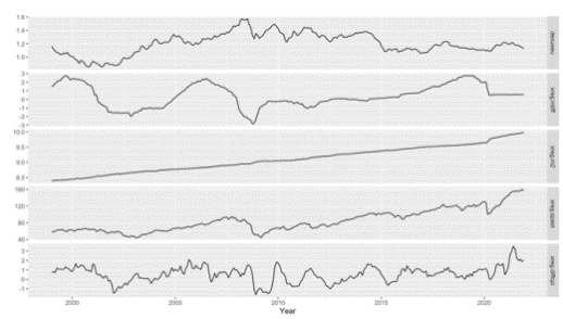
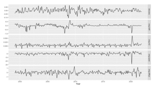
Figure 3: (a) Monthly and (b) one-order difference of the USD/EURO spot exchange rate.

Notes: Difference of the Immediate Interest Rate for USD-EURO, M2, US Total Share Prices, and Diff of CPI for USA/Euro area for each panel from top to bottom covering the training period from January 1999~December 2021.

5.2. Model Constructions

In this part, to avoid the complex discussion about the parameter selection procedures and focusing on the impacts of the regression variables, the automatic model constructions are used to build all ARIMA models.

Regular univariate ARIMA model. It is also worth noting that, with the only time series input, the auto.arima function in R-Studio provides a non-seasonal ARIMA, which made a very simple prediction. With a p-value of 0.09978, it presents a less symmetric normal distribution as displayed in Figure 4.

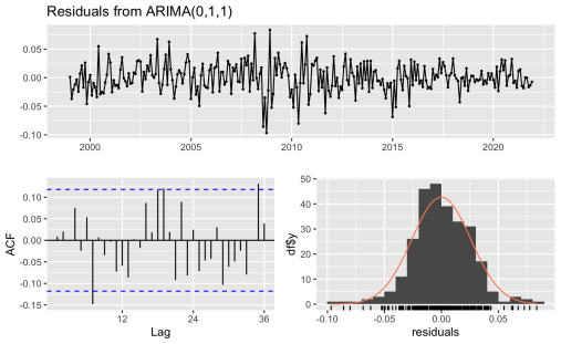
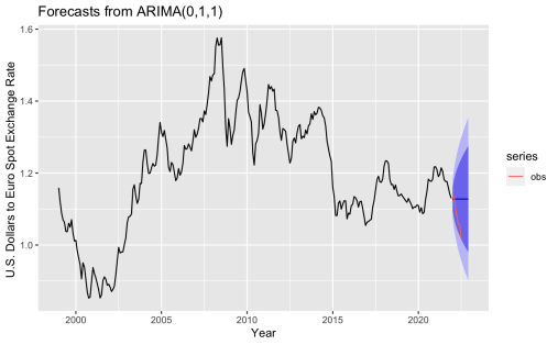
Figure 4: (a) The residual check and (b) foresting plots of the univariate ARIMA (0,1,1) model generated by auto.arima function.

Regression model with ARIMA errors. The auto.arima() function handles regression terms via the argument \( xreg \) specified and selects the best ARIMA model for the errors. It also forces all variables are differenced if differencing is required. Fortunately, all variables being used meet the differencing requirement according to the analysis in 5.1. In our study, \( xreg \) is specified with the training dataset of the four regression variables and finally the ARIMA [1,1,0] is generated thereafter automatically. The residuals check (Figure 5a), Ljung-Box test (omitted) and the ARIMA errors (Figure 5b) of the model reveal that the error of the model resembles a white noise series and ready for further forecasting.

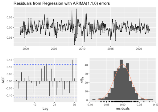
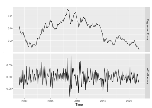
Figure 5: (a) The residual check and (b) regression errors ( \( {η_{t}} \) ) and ARIMA errors ( \( {ϵ_{t}} \) ) from the fitted model.

5.3. Forecasting and Evaluation

In this part, the univariate and multi-variate models are utilized for forecasting the USD/EURO spot exchange rates during the 8-month from January to August 2022. Their performances are evaluated.

Table 1: Experiments configurations.

Four experiments are designed as Table 1. UNI is the regular forecast of univariate ARIMA (0,1,1) model. However, it should be noted that when a regression model with ARIMA errors is utilized to forecast, predictors should be forecasted first and with their known values, the regression part and the ARIMA part of the model are forecasted jointly. In this study, three experiments are designed with different specifications of the predicted \( xreg \) . RE0 experiment is served as a benchmark result, which uses the observed values of all variables during the 8-month long forecasting period. In RE1, the \( xreg \) is predicted first by a simple forecasting method, random walk with drift, which sets the forecasts to be the value of the last observation. In RE2, the \( xreg \) is composed by the predicted values of all variables with their individual ARIMA models constructed separately and automatically.

The forecasts of the USD/EURO spot exchange rates during the 8-month from January to August 2022 from the four experiments are illustrated in Figure 6. It can be found that the UNI model has no ability to forecast the trend of the exchange rate, which implies that the regression model with ARIMA errors is of crucial importance for forecasting. RE0, the benchmark forecast, are almost perfectly fitted with the value and falling trend of the observed exchange rates, demonstrating the effectiveness of the ARIMA model with predictors input correct enough (the observed). RE1 with the predictors forecasted by the random walk does forecast the falling trend, but its forecasts are much lower than the observations. With all predictors predicted by auto.arima models constructed separately, the RE2 experiment forecasts the slow falling trend but the values are far from the lowest value approaching 1, the parity. In general, the regression model with ARIMA errors is capable of forecasting the historical change of the USD/EURO spot exchange rate. However, its performance totally depends on the quality of the predicted predictors, which are the four macroeconomic variables in this study.

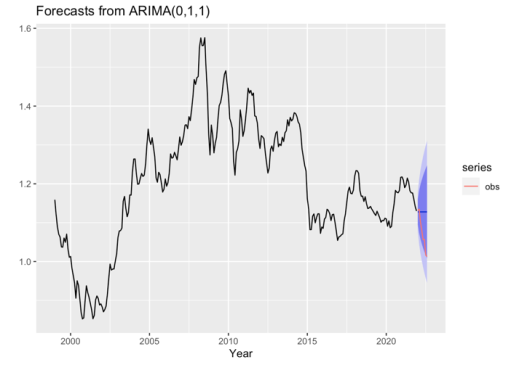
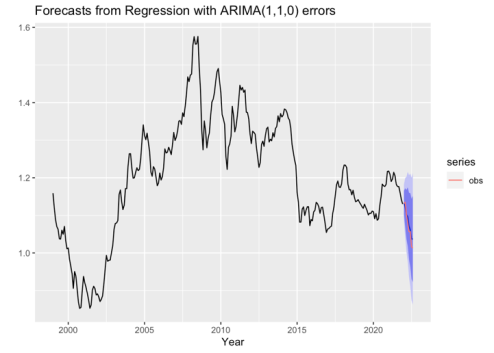
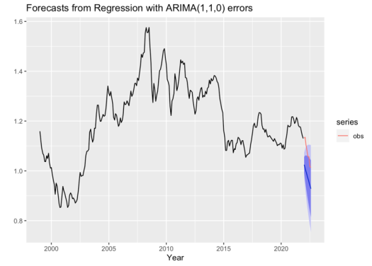
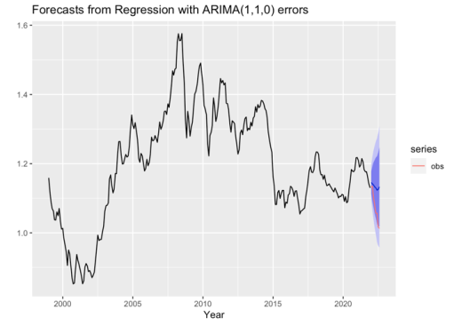
Figure 6: Forecasts of the USD/EURO spot exchange rates during the 8-month from January to August 2022 from the four experiments (a) UNI, (b) RE0, (c) RE1, and (d) RE2.

Note: Black lines are the time series of the exchange rate from the historical observations, the blue lines are the forecasts, red lines are the observations, and the shadows in light and deep purple represent the prediction intervals of 80% and 95% respectively.

6. Conclusions

Exchange rate forecasting is of great importance for both financial decision making and economic foreground judging. ARIMA model, as a long-developed classical statistical method, can be taken to do forecasts with fine accuracy, according to previous literatures. However, in the context of the plunge of the US/Euro Exchange Rate in 2022, the adequately data-based ARIMA model seems cannot obtain an approving prediction. Thus, to improve the performance and increase the applicability of ARIMA models in parallel contexts, four macroeconomic variables which are closely related to exchange rate forecasting in macroeconomic senses, are added as covariates to the initial ARIMA model. As a result, the multivariable ARIMA models have been demonstrated to predict the 2022's plunge event in a significantly improved accuracy. The comparison between RE1, RE2 and RE0 suggests that, the regression model with ARIMA errors is capable of forecasting the historical change of the USD/EURO spot exchange rate, while its performance totally depends on the quality of the predicted predictors, which are the four macroeconomic variables in this study. Therefore, with the consideration taken to the macroeconomic factors, ARIMA model itself, as a non-complex and non-multivariable hybrid model, can do a precise forecast likewise. The conclusion in this study can be used to solve similar problems in smeltable scenarios and enhance the performance and feasibility of these simple linear models on analyzing intricate real-world issues informingly. However, in the future study, the construction scheme of ARIMA model needs to be optimized furtherly. In addition to ARIMA model, other GARCH or VAR models can be tried to improve research methods; at the same time, for these macroeconomic variables, this paper also needs to consider the value of M2 and the total stock price in Europe. The model proposed in further research will be more conclusive, and the conclusion can be extended to more general research, which is persuasive.

References

[1]. Huang W, Lai K K, Nakamori Y, et al.: Forecasting foreign exchange rates with artificial neural networks: A review. International Journal of Information Technology & Decision Making, 3(01), 145-165(2004).
[2]. Dunis C L, Huang X: Forecasting and trading currency volatility: An application of recurrent neural regression and model combination. Journal of forecasting, 21(5), 317-354, (2002).
[3]. Ghalayini L: Modeling and forecasting the US dollar/euro exchange rate. International Journal of Economics and Finance, 6(1),194-207 (2014).
[4]. Akincilar A, TEMİZ İ, Şahin E: An application of exchange rate forecasting in Turkey. Gazi University Journal of Science, 24(4), 817-828 (2011).
[5]. Kamruzzaman J, Sarker R A. ANN-based forecasting of foreign currency exchange rates. Neural Information Processing-Letters and Reviews, 3(2): 49-58 (2004).
[6]. AsadUllah M, Bashir M A, Aleemi A R: Forecasting Euro against US dollar via combination of NARDL and Univariate techniques during COVID-19. Foresight, (2021).
[7]. Babu A S, Reddy S K: Exchange rate forecasting using ARIMA. Neural Network and Fuzzy Neuron, Journal of Stock & Forex Trading, 4(3), 01-05 (2015).
[8]. Weisang G, Awazu Y: Vagaries of the Euro: an Introduction to ARIMA Modeling. Case Studies In Business, Industry And Government Statistics, 2008, 2(1): 45-55.
[9]. Xu Z. Purchasing power parity, price indices, and exchange rate forcasts. Journal of International Money and Finance, 22(1), 105-130 (2003).
[10]. Hyndman R J, Athanasopoulos G. Forecasting: principles and practice. OTexts, (2018).
Cite this article
Zhu,Q. (2023). Forecasting the US Dollar/Euro Exchange Rate Based on ARIMA Model. Advances in Economics, Management and Political Sciences,15,371-380.
Data availability
The datasets used and/or analyzed during the current study will be available from the authors upon reasonable request.
Disclaimer/Publisher's Note
The statements, opinions and data contained in all publications are solely those of the individual author(s) and contributor(s) and not of EWA Publishing and/or the editor(s). EWA Publishing and/or the editor(s) disclaim responsibility for any injury to people or property resulting from any ideas, methods, instructions or products referred to in the content.
About volume
Volume title: Proceedings of the 2nd International Conference on Business and Policy Studies
© 2024 by the author(s). Licensee EWA Publishing, Oxford, UK. This article is an open access article distributed under the terms and
conditions of the Creative Commons Attribution (CC BY) license. Authors who
publish this series agree to the following terms:
1. Authors retain copyright and grant the series right of first publication with the work simultaneously licensed under a Creative Commons
Attribution License that allows others to share the work with an acknowledgment of the work's authorship and initial publication in this
series.
2. Authors are able to enter into separate, additional contractual arrangements for the non-exclusive distribution of the series's published
version of the work (e.g., post it to an institutional repository or publish it in a book), with an acknowledgment of its initial
publication in this series.
3. Authors are permitted and encouraged to post their work online (e.g., in institutional repositories or on their website) prior to and
during the submission process, as it can lead to productive exchanges, as well as earlier and greater citation of published work (See
Open access policy for details).