1. Introduction

The Federal Funds Rate is the interest rate at which banks lend or borrow overnight funds from each other, usually on an uncollateralized basis. It is also known as the "overnight rate" or the "target rate." The short target is an internal objective defined unilaterally by the Chairman of the Federal Reserve System by directives established at Federal Open Market Committee meetings (FOMC) [1].

The Federal Reserve can impact economic growth, inflation, and employment by altering the interest rate. If, for instance, raise the federal funds rate, it becomes more expensive for banks to borrow money, which can discourage lending and reduce economic activity.

The objective of this study is to use multiple linear regression estimated by OLS to create a predictive model for the federal funds rate in the U.S.. It minimizes the SSR between the observed data in the collection and the expected responses by linear approximation [2]. Several factors make linear regression beneficial for predicting the federal funds rate.

First, the relation between the federal funds rate and its influencing variables, including economic indicators and policy measures, is usually linear. This indicates that the rate is proportionate to the independent variables. For instance, if the unemployment rate rises, the rate may increase as well. Second, linear regression is a simple, well-known, and straightforward statistical procedure. It can offer a transparent and interpretable model of the relationship between the interest rate and variables, which helps determine how the pace will likely fluctuate in response to various economic conditions. When a linear model describes the connection between the variables well, linear regression can produce reliable predictions of the federal funds rate [3]. While other statistical methods may be more appropriate in some instances, linear regression is frequently a reasonable starting point for estimating the federal funds rate. It can provide valuable insights into its influencing elements.

The empirical result shows that the federal funds rate is positive in connection with the monetary base change rate, treasury yields, and CPI change rate but negatively impacted by the unemployment rate and real GDP growth rate.

The Federal Funds Rate is optimistic about the monetary base change rate because the Federal Reserve can use its ability to buy or sell government securities to affect how much money there is in the economy. By increasing the monetary base, the Federal Reserve can circulate more money, leading to lower interest rates. Conversely, if the Federal Reserve reduces the economic base, It could restrict the money supply and raise interest rates.. The Federal Funds Rate is also positively associated with treasury yields, which are the interest rates that the government pays on its debt. When the Federal Reserve raises the speed, it can result in higher treasury yields, as investors demand a higher return on their investments. The rate is positively related to the CPI change rate because a higher rate can lead to increased inflation. When the Federal Reserve raises the speed, it can result in higher borrowing costs for businesses and consumers, leading to higher prices for goods and services. Besides, the unemployment rate and real GDP growth rate hurt the rate. The Federal Reserve often uses the federal funds rate to help stimulate economic growth and reduce unemployment [4]. The Federal Reserve may cut the pace to boost economic activity and promote job creation if unemployment is high or GDP growth is slow. In contrast, if both the unemployment and GDP growth rates are low, the Federal Reserve may increase the speed to curb inflation and maintain economic stability.

2. Ordinary Least Squares Regression

Ordinary least squares (OLS) regression is a popular tool for finding the coefficients of linear regression equations that depict the relationship between independent variables and a dependent variable. The least squares represent the minimum square error (SSE) [5].

The OLS regression for a model with five variables may be expressed as:

\( Y={β_{0}}+\sum _{1}^{5}{β_{j}}*{X_{j}}+ε \) (1)

Where Y is the dependent variable, β₀, is the model intercept, X_j corresponds to the jth explanatory variable of the model (j = 1 to 5), and e is the random error with expectation 0 and variance σ².

With 754 observations, the estimate of the expected value of the dependent variable Y for the ith observation is provided by:

\( {Y_{i}}={β_{0}}+\sum _{1}^{p}{β_{j}}*{X_{ij}} \) (2)

The goal of OLS regression is to find the results of b₁ to b₇₅₄ that minimize the SSR, which can be expressed mathematically as:

\( \sum _{1}^{754}{(y - {b_{j}}*x)^{2}} \) (3)

For multiple linear regression models with multiple independent variables, the OLS equation takes the form:

Y = \( \sum _{1}^{754}({b_{j}}*{x_{j}}) \) (4)

Where x are the independent variables and b are the corresponding coefficients. The goal is still to minimize the SSR. Once the coefficients have been estimated, the OLS model can be used to create predictions for the dependent variable.

3. Data Description

The Federal Reserve Economic Data and the U.S. Bureau of Labor Statistics provided the model's information. The frequency of the data is monthly (the original, accurate GDP growth rate data is annual. To make it conform to the structure of the model, I divided the yearly growth rate by 12 to obtain the average number to fill the chart), and the sample size is 754 individuals.

The independent variables chosen for the model are the monetary base change rate, treasury yields, unemployment rate, CPI change rate, and real GDP growth rate from January 1960 to October 2022. These are all economic indicators that can be useful in predicting the rate. A sample of the dataset's first five rows is shown in Table 1:

Table 1: Initial data sample: a preview of the dataset.

The monetary base change rate refers to the rate of change in the total amount of currency in circulation and banks' reserves. This can be an essential factor in predicting the pace because the Federal Reserve uses it as one of its tools. It can be used to affect the amount of money available in the economy and, in turn, the level of inflation [6]. The Federal Reserve may be trying to stimulate the economy by expanding the money supply if the monetary base is growing quickly. This could increase the federal funds rate [7].

Treasury yields describe the rate of return that investors receive on their investments in U.S. government bonds. These yields can be an essential factor in predicting the momentum because they are closely related to the economy's general interest rate level. If Treasury yields are rising, this may be a sign that investors expect the Federal Reserve to raise the rate in the future. Figure 1 shows the evolution of Treasury Yields and federal funds rate from 1960 to 2022.

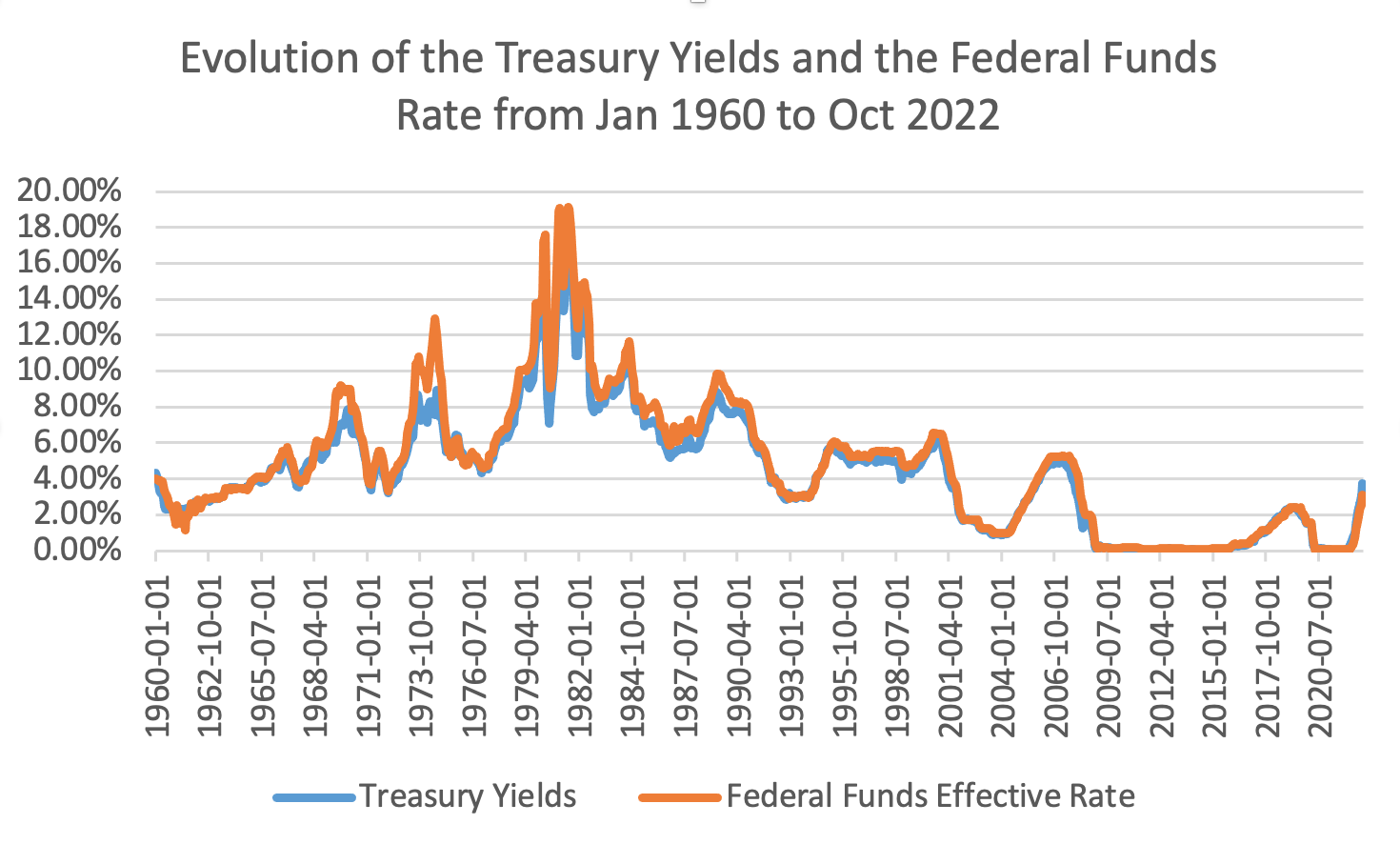
Figure 1: Treasury yields and federal funds rate evolution: 1960-2022.

The unemployment rate is the proportion of the labor force that is unemployed but actively looking for jobs. It can be a vital factor in predicting the pace because the unemployment rate is a standard indicator of the labor market's health used by the Federal Reserve. If the unemployment rate is high, this can be a sign that the economy is not performing well, which may lead the Federal Reserve to lower the rate to stimulate economic activity.

The Consumer Price Index (CPI) change rate is a measurement of the average price level of goods and services that households typically purchase. This can be an important factor in predicting the rate because the Federal Reserve uses the CPI as one of its primary measures of inflation. If the CPI is rising rapidly, this may be a sign that the economy is experiencing high levels of inflation, which may result in raising the rate to contain inflation.

Moreover, the real GDP growth rate refers to the change rate in a country's gross domestic product (GDP), adjusted for inflation. This can be an essential factor in predicting the pace because the Federal Reserve often uses the GDP as an indicator of the economy overall [8]. If the GDP is increasing, this may be a sign that the economy is performing well, and to keep inflation under control, the Federal Reserve may boost the rate.

4. Empirical Results

The following table can be obtained by performing OLS regression based on the data reviewed in the preceding section:

Table 2: OLS regression results table.

As shown in Table 2, this table contains the results of a multiple regression analysis. The numerous R-value of 0.99 indicates that the independent and dependent variables have a solid linear connection. The R Square value of 0.98 indicates that the predictor variables explain about 98% of the variance of the federal funds rate. Also, the adjusted R Square value of 0.98 is comparable to the R Square value, but it considers the number of predictors and adapts the R Square value accordingly [9]. The standard error value of 0.0049 represents the precision of the model's prediction.

The ANOVA data in Table 3 shows the results of a hypothesis test for the model's overall fit. The F-value of 8437.44 is relatively high, indicating that the model is a good fit for the data. The p-value of 0.00022 is less than 0.05, which means that the model is reliable and the independent variables substantially impact the dependent variable.

Table 3: ANOVA table for OLS regression.

The coefficients table shows the estimated coefficients for each variable in the model, along with the standard error, t-statistic, and p-value for each coefficient. Each coefficient's p-value is less than 0.05, signifying that each independent variable has a highly relevant impact on the dependent variable. The 95% and 99% confidence intervals for each coefficient provide a range of values within which the actual coefficient is likely to fall.

The general form of the regression equation is Federal Funds Rate = intercept + (coefficient for Monetary Base Change Rate * Monetary Base Change Rate) + (coefficient for Treasury Yields * Treasury Yields) + (coefficient for Unemployment Rate * Unemployment Rate) + (coefficient for CPI Change Rate * CPI Change Rate) + (coefficient for Real GDP Growth Rate * Real GDP Growth Rate)

Using coefficients from the table, the equation for regression can be expressed as follows:

Y = 0.0013 + 0.0306 * X₁ + 1.1432 * X₂ - 0.0373 * X₃ + 0.2638 * X₄ - 0.8037 * X₅ (5)

5. Prediction

This section aims to split the dataset into two parts (training set and test set), create a regression model with one piece, and test the model's accuracy with the other part. The training set includes 600 samples from January 1960 to December 2009, and the test set consists of the rest, 154 individuals.

Based on the training set, the new regression table can be obtained:

Table 4: Predictive regression results table.

As shown in Table 4, we can accept independent variables if the t-stat is more significant than 2 or the p-value is less than 0.05 at the 95% level of significance [10]. Using the coefficients from the table, the regression equation can be written as follows:

Y = 0.0034 + 0.0417 * X₁ + 1.1690 * X₂ - 0.0923 * X₃ + 0.2743 * X₄ - 1.0137 * X₅ (6)

As shown in Figure 2, by analyzing the test set and applying the aforementioned equation, we can calculate the accuracy rate of the model. If the error of the estimated value is within 0.005, then we can consider the data to be accurate. The result is that 107 out of the 154 samples in the test set are in the range. The accuracy rate is approximately 69.48%.

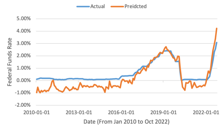
Figure 2: Comparison of predicted and actual federal funds rate.

6. Concluding Remarks

In conclusion, our study has shown that linear regression can help predict the federal funds rate in the United States. By using data on various economic and financial indicators, including the monetary base change rate, Treasury yields, the CPI change rate, the unemployment rate, and the real GDP growth rate, we were able to fit a linear regression model that accurately captured the connection between the speed and these variables. Our model demonstrated good predictive performance, with an R-squared value of 0.98 and an accuracy rate of 69.48%. These results provide valuable insights into the factors influencing the rate and will interest many academic and practical audiences.

References

[1]. Hamilton, J.D., Jorda, O. (2002) A Model of the Federal Funds Rate Target. J. Political Economy, 110(5), 1135–1167.
[2]. Ferrando, L., et al. (2015) Interest Rate Sensitivity of Spanish Industries: A Quantile Regression Approach. The Manchester School, 85(2), 212–242.
[3]. Estrella, A., Mishkin, F.S. (1998) Predicting U.S. Recessions: Financial Variables as Leading Indicators. The Review of Economics and Statistics, 80(1), 45–61.
[4]. Labonte, M., Makinen, G.E. (2008) Monetary policy and the Federal Reserve: current policy and conditions. Congressional Research Service, Library of Congress.
[5]. Seber, G.A.F., Lee, A.J. (2012) Linear regression analysis. John Wiley & Sons.
[6]. Campbell, J.R., et al. (2012) Macroeconomic effects of federal reserve forward guidance. Brookings papers on economic activity, 1-80.
[7]. Moore, B.J. (1983) Unpacking the Post Keynesian Black Box: Bank Lending and the Money Supply. Journal of Post Keynesian Economics, 5(4), 537–556.
[8]. Faust, J., Swanson, E.T., Wright, J.H. (2004) Do Federal Reserve Policy Surprises Reveal Superior Information About the Economy? Contributions to Macroeconomics, 4(1), 10.
[9]. Maier, H., Morgan, N., Chow, C.W.K. (2004) Use of artificial neural networks for predicting optimal alum doses and treated water quality parameters. Environmental Modelling & Software, 19(5), 485-494.
[10]. Kim, J.H. (2019) Multicollinearity and misleading statistical results. Korean Journal of Anesthesiology, 72(6), 558-569.
Cite this article
Qiu,T. (2023). Predicting the Federal Funds Rate: A Linear Regression Analysis. Advances in Economics, Management and Political Sciences,20,57-62.
Data availability
The datasets used and/or analyzed during the current study will be available from the authors upon reasonable request.
Disclaimer/Publisher's Note
The statements, opinions and data contained in all publications are solely those of the individual author(s) and contributor(s) and not of EWA Publishing and/or the editor(s). EWA Publishing and/or the editor(s) disclaim responsibility for any injury to people or property resulting from any ideas, methods, instructions or products referred to in the content.
About volume
Volume title: Proceedings of the 2023 International Conference on Management Research and Economic Development
© 2024 by the author(s). Licensee EWA Publishing, Oxford, UK. This article is an open access article distributed under the terms and
conditions of the Creative Commons Attribution (CC BY) license. Authors who
publish this series agree to the following terms:
1. Authors retain copyright and grant the series right of first publication with the work simultaneously licensed under a Creative Commons
Attribution License that allows others to share the work with an acknowledgment of the work's authorship and initial publication in this
series.
2. Authors are able to enter into separate, additional contractual arrangements for the non-exclusive distribution of the series's published
version of the work (e.g., post it to an institutional repository or publish it in a book), with an acknowledgment of its initial
publication in this series.
3. Authors are permitted and encouraged to post their work online (e.g., in institutional repositories or on their website) prior to and
during the submission process, as it can lead to productive exchanges, as well as earlier and greater citation of published work (See
Open access policy for details).