1. Introduction

The epidemic that raged from 2019 to 2023 is still fresh in the memory of most shareholders and investors. The financial market has evaporated more than trillion yuan, especially the tourism, catering and other industries have suffered immeasurable losses, which fully shows that the capital market is a cruel battlefield vulnerable to the stimulation of external factors such as civic sentiment. However, with the continuous development of the economic system and financial system towards marketization, China's financial market innovation continues to develop. The scale of the financial market continues to expand, and the market coverage and influence continue to increase. The financial market continues to reform and its functions are increasingly improved. The structure is optimized, and the multi-level financial market system is being formed [1]. With the rapid development of today's big data, more and more investors begin to learn foreign advanced investment theories, and use some financial models and statistical theories to quantify and visualize risks and returns. Nowadays, investment transactions in domestic and foreign financial markets are changing from subjective transactions based on traditional technical analysis to quantitative strategic transactions based on computer programs [2]. The application of statistical arbitrage strategy based on paired trading in China's futures market has been extensively studied, while the research on paired trading in China's stock market in the past five years is relatively small, and the effectiveness of paired trading needs to be verified.

Paired trading originated from the sister pair trading strategy adopted by Jesse Lauriston Livermore in the 1920 investment event [3]. Its principle is to find two stocks with similar stock price trends, and use data (e.g., price difference and price ratio) to find out the time point deviating from the normal range to short the assets with relatively high prices. Subsequently, one can buy the assets with relatively low prices for arbitrage, build positions when the price deviation is large, and close positions when the price deviation is small, so as to earn profits.

There have been a number of studies in China about matching the A-share market. Wang et al. selected CSI 300 component stocks as the stock pool and used the index to measure the stock price difference as the stock matching standard [4]. The results showed that this strategy was effective and could make stable profits in the Chinese market. Zhu selected the constituent stocks of the Shanghai 180 Index as the stock pool and found the optimal threshold for opening and closing positions by comparing the portfolio returns when different thresholds were selected [5]. Tang et al. selected 50 component stocks of Shanghai Stock Exchange as the stock pool [6], used the daily closing price data of three years from 2014 to February 17 for co-integration matching, and used support vector machine regression to verify the effectiveness of the model [7].

In this paper, the daily closing prices of the CSI300 and CSI500 in the past two years are used as the data set, and the daily closing prices and returns are paired according to Pearson correlation coefficient. The trading data of the 20 portfolios with the highest correlation coefficient from August 10, 2021 to August 10, 2022 are trained for matching trading, and the best parameters obtained from the training are applied to the market data from August 11, 2022 to February 9, 2023 for back testing, four groups of 20 stock pairs can obtain an annualized yield of 23%.

2. Data & Method

Following previous study, combining the current market situation and previous research results, this paper proposes the following research scheme. First, this article uses the CSI 300 and CSI 500 to build the initial stock pool, and then eliminate the stocks with missing values, suspension and listing after 2021. Then, we can calculate the daily rate of return and daily closing price by using the Person correlation coefficient. On this basis, one can obtain the 20 pairs with the highest closing price correlation number, the 20 pairs with the lowest closing price correlation coefficient, the 20 pairs with the highest yield correlation coefficient and the 20 pairs with the lowest yield correlation coefficient.

After obtaining 80 pairs of matching results, for the two stocks in the pairing result, the authors take August 10, 2021 to August 10, 2022 (inclusive) as the training period. and use the closing price data of the training period to carry out zero intercept regression, and the slope term obtained by zero intercept regression β₁ as the price multiplier between two stocks, calculate the relative price difference Z= β₁X-Y, calculate the relative price difference Z into the Bollinger band channel, get the trading signal, and calculate the yield.

We use multiple sets of mean line period values and standard deviation values to draw the Brin band, then find out the most suitable parameters for the Brin band drawing of the stock price data during the training period. Then, the authors apply the parameters to the stock data from August 10, 2022 to February 9, 2023 to carry out the paired trading test, and calculate the yield, volatility, Sharp ratio, and maximum withdraw. The four rectangles at the left of the Fig. 1 show the main steps of the research process. The blue downward shears show the sequence of main steps. The rectangles at the right of the main steps explains the method and the material, and the rectangles after the second red shears explain the key method of every steps.

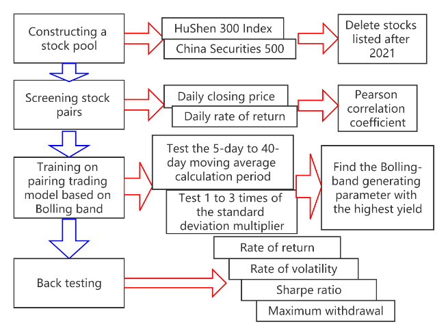
Figure 1: The whole research process. The rectangle in Fig.1 represents a step or method. The blue cut head in Fig. 1 represents the before and after relationship between the steps. The red cut head in Fig.1. indicates the key details in the method.

2.1. CSI300 & CSI500

In order to verify the accuracy of matching transactions, this study selects a group of sufficiently representative stocks as the stock pool. This paper selects two stock pools of CSI 300 and CSI 500, a total of 800 stocks, and removes stocks with suspended trading, ST and missing values at the daily closing price. CSI 300 is a simulated index futures launched by CICC, and a large number of domestic investors actively participate in the simulation trading, learning the new trading rules of stock index futures. CSI 300 simulates the development features and lessons, which after the futures trading [8]. The CSI 500 is the CSI 500 futures index, which was listed on April 16, 2015 during the 2015 stock disaster and was specifically set up for the GEM and SME board [9]. The reasons for selection are as follows. The CSI 300 have strong liquidity and large scale, and the industry distribution of CSI 300 is similar to the reality, which is representative [7]. Besides, CSI500 is a non-ST, non-suspended stock, and the company has no major violations of laws and regulations within one year, and there are no major issues in the financial report [10]. In January 2023, the number of listed stocks in China's A-share market was 4997, and the stock pool consisting of CSI300 and CSI500 accounted for 16% of the total number of stocks in the market. Compared with the method of using CSI100 or CSI300 as the stock pool in other studies, the stock pool selected in this paper is larger and more representative. The stock trading data used in the study, including the list of CSI300, the list of CSI500 and the daily trading data of stocks, are all from www.baostock.com, which is a network data platform providing Python api.

2.2. Screen Stock Pairs

Pearson correlation coefficient is a method of calculating linear correlation proposed by British statistician Pearson in the 20th century. The specific calculation formula is as follows:

\( {ρ_{X,Y}}=\frac{N∑XY-∑X∑Y}{\sqrt[]{N∑{X^{2}}-{(∑X)^{2}}}\sqrt[]{N∑{Y^{2}}-{(∑Y)^{2}}}}\ \ \ (1) \)

Here, N is the number of samples in population X, and the number of samples in X is equal to the number of samples in Y. Pairing transactions need to use stock portfolios with similar trends. This paper uses Pearson correlation coefficient to pair all stocks in the stock pool, and calculates the correlation between daily closing price and daily yield. In order to compare the different effects of different stocks on the calculation method, four experimental groups are designed in this paper. We take the last 20 from the correlation coefficient of daily closing price, i.e., the 20 groups of stock pairs with the strongest negative correlation of daily closing price. We take the top 20 from the correlation coefficient of daily closing price, i.e., 20 groups of stock pairs with the strongest positive correlation of daily closing price. We also take the last 20 from the correlation coefficient of daily return, i.e., the 20 groups of stock pairs with the strongest negative correlation of daily return. We choose the top 20 from the correlation coefficient of daily return, i.e., the 20 groups of stock pairs with the strongest positive correlation of daily return. Finally, the authors set up four experimental groups to test the difference between the two matching methods of the correlation coefficient based on the closing price and the correlation coefficient based on the yield, as well as the difference between the positive correlation and the negative correlation.

2.3. The Process of Bolling Trading

Bollinger band channel strategy is a classic channel strategy. It combines the standard deviation and average line, using the average line to constrain the smoothness of the channel, and using the standard deviation to constrain the width of the channel [7]. The Bolin Belt is composed of four lines: price line, resistance line, support line and average line. The average line is the average line of the price line, which is generally the 20-day average line. The resistance line is generally the average line minus twice the standard deviation, and the support line is generally the average line plus twice the standard deviation. The price line will move in the channel between the resistance line and the support line. When the price line crosses the resistance line, it will generally fall back. When the price line crosses the pressure line, it will generally rise. Bolin line is intuitive, flexible, and trendy, so it is favored by a large number of investors [11].

In this paper, we use the Bollinger band to constrain the trend of the relative price difference and judge the trading signal. Traditional paired trading uses fixed moving average to judge the trading signal, and the Bollinger band is more flexible. Zero intercept regression is a method of fitting independent variable Y into regression equation \( {Y_{i}}=β{X_{i}}+{u_{i}} \) by least square method, where β is the slope after fitting and ui is the residual term.

\( β=\frac{∑{X_{i}}{Y_{i}}}{∑{{X_{i}}^{2}}}\ \ \ (2) \)

In this paper, the zero intercept regression is used to calculate the price multiples of two stocks in the stock pair, and then the relative spread Z=β_1X-Y is calculated. The trading process of this paper is to first buy 1,000,000 shares of one stock in the pair as stock X, then calculate the relative spread Z=β_1X-Y, and calculate the Bolling band channel according to the relative spread. When the relative spread crosses the support line, if there is stock X in the position, sell stock X and buy stock Y in the full position. When the relative spread crosses the resistance line, if there is stock Y in the position, sell stock Y in the full position and buy stock X.

2.4. Backtesting Evaluations

In this paper, three calculation methods are used to evaluate the back test. Using zero intercept regression to calculate the price multiplier of two stocks during the training period. The result is coefficient β=3.0659, standard error = 0.027, t = 115.637. Rate of return is the simplest and most intuitive evaluation method, and its calculation formula is: rate of return = income/principle. In this paper, the principal is set for initial purchase of 1.000,000 shares X the total price, and finally the cumulative rate of return from the beginning to the end is calculated. Volatility is the standard deviation of the rise and fall of assets over a period of time. Volatility reflects the risk level caused by the uncertainty of asset return. The higher the volatility, the higher the risk level caused by uncertainty of asset return, and the lower the volatility, the lower the risk level caused by uncertainty of asset return [7]. Sharpe ratio is a commonly used index to measure the return and risk of portfolio, and its core idea is select the fund with the largest expected return when the given risk level is similar, and select the fund with lower risk level when the return is similar. This helps people to jump out of the misunderstanding of high risk and high return. The calculation formula of sharp ratio is Sharpe Ratio=[E(Rp)－Rf]/σp. Here, E(Rp) represents the average growth rate of the fund’s net value and Rf represents the risk-free interest rate, and the difference between them is divided by the portfolio. The standard deviation of the rate return gives the total excess return per unit risk. It is not difficult to see from this formula that When SR is less than zero. The growth rate of the fund is less than the risk-free interest rate, which has no investment significance. When SR is greater than 1, it means that the excess return is greater than the risk, and when SR is less than 1, the excess return is less than the risk. The greater the sharp ratio, the more excess return and the greater the investment value. Maximum retracement refers to the maximum value of the retracement amplitude of the rate of return when the product net value reaches the lowest point at any historical time point in the selected period. That is, the worst situation that may occur after buying a product is used to measure the ability of products such as funds to resist wind and industrial risks. The following is the formula for calculating the maximum retracement: Max drawdown=max(Px-Py)/Px.

3. Results & Discussion

3.1. Pairing of Stocks

Using Pearson correlation coefficient, the daily closing price and daily return rate of each stock pool are paired in pairs, and the results are obtained as shown in Table. 1 (for each experiment group, the absolute value of correlation coefficient is highest). Every line in the table shows the last 1 pair or the first 1 pairs of every pairing group, with the two coefficient of daily closing price and daily rate of return. Tasking two stocks, sh600809 and sz000568, for example, one can draw their trend charts, which shows that there is indeed a similar trend between the two stocks. According to the stock information (seen from Fig. 2), sh600809 is Shanxi Fenjiu and sz000568 is Luzhou laojiao, both of which are liquor stocks. Obviously, the two stock have peak and valley at the same time.

Table 1: The pairing result of every experimental groups.

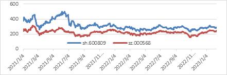
Figure 2: The daily closing price of sh6000809 and sz000568. The y-axis shows price of every stock, and the x-axis shows date.

3.2. Training Pair Trading

The authors take the period from August 10th, 2022 as the training period. Take sh600809 and sz000568 for example, the authors calculate the training period price difference with formula Z=β1X-Y, and draw the Bollinger band channel. As show in Fig. 3, the Bollinger band channel chart with a 20-day moving average and a standard deviation of 2 times: multiple sets of moving average drawing parameters and standard deviation ratio are applied to the drawing process of Bollinger bands,

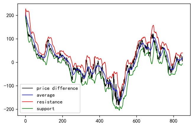
Figure 3: A The Bollinger bands of training process for sh600809 and sz000568. The black line shows the relative price of the two stocks, and the blue line is the 20 days average line, the red line is the average line plus 2 times of standard deviations, the green line is the average line minus 2 times of standard deviations.

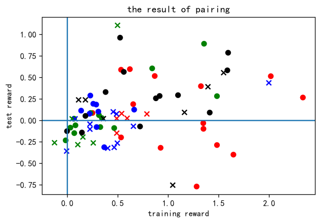
Figure 4: The result of pairing from every training groups.

3.3. Backtesting Evaluations

Several groups of parameters with the highest yield obtained in the training process of matching trading are applied to the trading data from August11,2022 to February9,2023, and the matching trading is carried out again, and the yield, volatility, sharp ratio and maximum retracement are obtained. The Fig. 4 shows the test results of 80 pairs. Different colors in the picture represent different experimental groups. The green dots represent the 20 stock pairs with the strongest negative daily return correlations. The red dots represent the 20 stock pairs with the strongest positive daily return correlations. The black dots represent the 20 stock pairs with the strongest negative daily closing price correlations. The blue dots represent the 20 stock pairs with the strongest positive daily closing price correlations. The X in the figure indicates that the optimal Bollinger Band matching parameters of the stock portfolio are special, so there is no matching transaction during the training period, that is , the maximum rate of return is obtained only by holding stock X. The “.” The Table. 2 indicates that there is a matching transaction during the training period.

Table 2: The average reward of training process and back testing process, and the volatility, Sharpe ratio, max drawdown ratio in back test process.

3.4. Mean Value Analysis

In terms of yield, the 20 stock pairs with the strongest positive correlation of daily yield obtained the highest yield among the four experimental groups during the training period. However, the 20 stock pairs with the strongest negative correlation between daily closing prices obtained the highest yield among the four experimental groups during the test period. It shows that in this experiment, the negative correlation of closing price is the best. In terms of volatility and maximum retracement, the 20 stock pairs with the strongest negative correlation between daily closing prices have the highest volatility and maximum retracement during the test period. On the other hand, the results of the daily rate of return experimental group show that both experimental groups have lower volatility and maximum retracement during the test period. In this experiment, the risk of negative correlation trading with closing price is the greatest. In terms of sharp ratio, the 20 stock pairs with the strongest positive correlation of returns have the highest sharp ratio, followed by the 20 groups with the strongest negative correlation of returns, the 20 groups with the strongest positive correlation of closing prices and the 20 groups with the strongest negative correlation of closing prices. Among them, the 20 stock pairs with the strongest negative correlation between closing prices even obtained negative sharp ratio. It indicates that in this experiment, the 20 stock pairs with the strongest positive correlation in returns have achieved the best balance between return and risk.

3.5. Quantitative Analysis of Negative Values

In terms of yield, only the 20 stock pairs with the strongest positive correlation in yield achieved a loss of 0 pairs in the test period, while only the 20 stock pairs with the strongest negative correlation in closing prices achieved a loss of 4 pairs in the test period, and the number of negative returns in the other three experimental groups was close to half. It shows that the risk of Bollinger Band pairing transaction is the smallest among the 20 stock pairs with the strongest negative correlation between closing prices. In terms of sharp ratio, the four experimental groups have a large number of negative numbers. Among them, the 20 stock pairs with the strongest positive correlation between daily closing prices have the most negative values, indicating the highest risk (seen from Table. 3).

Table 3: The number of below-zero value of training reward, test reward and sharpe ratio from every training groups.

4. Conclusion

To sum up, based on the stock data of China A-share market from August 10, 2021 to February 9, 2023, it is feasible to screen stock pairs by using the correlation coefficient of daily closing price and daily return rate. We carry out the quantitative investment strategy of matching trading training based on Bollinger Band, which can obtain the highest annualized return rate of 23%. Among them, the stock portfolio with the strongest negative correlation of daily closing price can get the highest return, while the stock portfolio with the strongest positive correlation of daily return is least risky. Compared with previous studies, it is found that the research in this paper has the following limitations. Primarily, the screening of the stock pool only considers whether it is listed after 2021, and does not consider the issue of ST mark. In addition, the transaction costs is ignored. Moreover, the transaction data is based on daily closing prices. Compare with time-sharing transaction data, the daily closing prices are lagged. For further research, more complex trading orders can be used, and the returns of the same trading strategy can be tested in different time segments. Overall, these results offer a guideline for Pair Trading using Bollinger Bands as the method of Trading signal judgement.

References

[1]. Bi, L., Zhu, B.: Current Situation and Development of Chinese financial market. Consumer Guide 16, 1, (2008).
[2]. Wen, X.: Research on high-frequency Quantitative Trading Strategy Based on Deep Reinforcement Learning. Modern Electronic Technology, 46(2), pp. 125⁃131 (2023).
[3]. Li, H.: Construction of Statistical Arbitrage Interval Based on Bank Stocks, Improvement and Application of Bollinger Belt, Guangdong University of Finance and Economics (2021).
[4]. Wang, C., Lin, B., Zhu, L.: Matching trading strategies based on stock price differences. Journal of Beijing University of Technology (Social Sciences Edition), 1, pp. 71-75 (2013).
[5]. Zhu, Y.: Research on paired trading of Shanghai 180 Index Component Stocks based on regression and Co-integration method. East China Normal University (2015)
[6]. Tang, L., Xu, Q., Luo, W.: Research on stock Matching based on Co-integration. Time Finance, 31, pp. 69-71 (2013).
[7]. Zhao, Y X.: Research on pairing trading strategy based on Shanghai and Shenzhen 300 Component Stocks. Lanzhou university (2022).
[8]. Xing, T., Zhang, G.: An empirical study on the linkage effect of stock index futures on spot market in China: Based on the analysis of CSI 300 simulation index futures data. Research on Financial Issues 4, 7 (2010).
[9]. Liu, C., Wang, Y.: Dynamic impact of Stock index futures on Stock Index during Stock market Crash in 2015: Based on the var model of China Securities 500 Stock Index Futures and Stock index. Journal of Guizhou Normal University, 32(8), 6 (2016).
[10]. Xiao, Y.: Based on Fama - French choose a strategy of three factor model research. Shanghai jiaotong university (2015).
[11]. Song, G.: Cloth forest quantitative trading channel statistical arbitrage strategy research. Guangdong university of finance and economics (2019).
Cite this article
Li,Y.;Song,X.;Yan,X. (2023). Analysis of Paired Trading Strategies Based on Boll Bands. Advances in Economics, Management and Political Sciences,23,259-267.
Data availability
The datasets used and/or analyzed during the current study will be available from the authors upon reasonable request.
Disclaimer/Publisher's Note
The statements, opinions and data contained in all publications are solely those of the individual author(s) and contributor(s) and not of EWA Publishing and/or the editor(s). EWA Publishing and/or the editor(s) disclaim responsibility for any injury to people or property resulting from any ideas, methods, instructions or products referred to in the content.
About volume
Volume title: Proceedings of the 2023 International Conference on Management Research and Economic Development
© 2024 by the author(s). Licensee EWA Publishing, Oxford, UK. This article is an open access article distributed under the terms and
conditions of the Creative Commons Attribution (CC BY) license. Authors who
publish this series agree to the following terms:
1. Authors retain copyright and grant the series right of first publication with the work simultaneously licensed under a Creative Commons
Attribution License that allows others to share the work with an acknowledgment of the work's authorship and initial publication in this
series.
2. Authors are able to enter into separate, additional contractual arrangements for the non-exclusive distribution of the series's published
version of the work (e.g., post it to an institutional repository or publish it in a book), with an acknowledgment of its initial
publication in this series.
3. Authors are permitted and encouraged to post their work online (e.g., in institutional repositories or on their website) prior to and
during the submission process, as it can lead to productive exchanges, as well as earlier and greater citation of published work (See
Open access policy for details).