1. Introduction

As we all know, in the process of venture capital investment, not every project can succeed. Thus, how to allocate the limited sources to achieve the goal of risk diversification and profit maximization is always an interesting issue in the financial area. In 1952, Markowitz introduced the mathematical statistics method to the study of portfolio selection, and for the first time analyzed the selection of the optimal portfolio in detail from the perspective of trade-off between return and risk. [1,2].

Since Markowitz's mean variance theory laid the foundation for current port-folio theory, research on portfolio theory has achieved many results and progress. For example, Lin and He studied the application of VaR model and CVaR model in portfolio construction and argued that CVaR model improved the effect of portfolio [3]. Considering the practical constraints such as V-type transaction costs, the researchers constructed a consistent mean CVaR credibility portfolio model [4]. A new efficient multi-objective portfolio optimization algorithm called 2-phase NSGA II algorithm is developed then and the results excelled in the comparison as well, etc [5].

Besides, there are many examples of machine analysis for stock investment portfolio. For example, Liu and Zhou used the adaptive lasso method to construct a sparse investment portfolio, and the results showed that the stock index was to some extent predictable [6]. Yin proposed a hybrid prediction method based on random forest, support vector regression and short-term memory network models, and constructed a risk index to improve the traditional mean variance (MV) model [7]. Zhang introduced the prediction residual of ARIMA into AT-LSTM and the experimental results showed that the combined model improved the pre-diction accuracy [8]. Zhang skipped the prediction step, and directly optimized the weight of the investment portfolio by updating model parameters [9]. To sum up, application of mean-variance optimization is still limited and deserve more investigations.

This paper connects ARIMA and mean-variance to broaden the application of ARIMA model and mean-variance analysis. To the best of the author’s knowledge, this paper embraces the following contributions and research to the literature. First, this paper collected the returns of five stocks through Tushare data and tested the stability of the data. Then, this paper made ARIMA related predictions. Next, this paper used a mean variance model to construct an investment portfolio based on the predicted return. Finally, a comparison is made be-tween the proposed model and the benchmark model.

2. Data

The data of this paper comes from Tushare Finance (https://www.tushare.pro/.com), and this paper selects the representative enterprises of the above five industries as examples, Moutai, Baosteel, Yidong, Dongfeng, Ping’an. The stock codes are 600519.SH, 600019.SH, 600941.SH, 600006.SH, 601318.SH, respectively. The reason is that these five enterprises are basically one of the most common brands in the Chinese market, which can rep-resent the level of this industry, or have good profitability in the past. And most importantly, investors are more willing to choose these stocks.

The closing price data of the latest year, from March 15th, 2022, to March 20nd 2023, is chosen and 247 pieces of data were collected. This paper divides these data into two parts. Firstly, using 217 pieces of data from March 15th, 2022, to February 6th, 2023, to make ARIMA predictions, and 30 pieces of data from February 7th, 2023, to March 17th, 2023, to find the optimal portfolio. After analyzing and calculating these data, the basic information obtained in this paper is as follows in Table 1, Table 2 and Table 3, respectively.

Table 1: Descriptive statistics of the daily return of the 5 stocks.

Table 2: Correlation matrix of returns of 5 stocks.

Table 3: Covariance matrix of returns of 5 stocks.

As shown in the tables above, Moutai has the highest average yield and the smallest standard deviation. The lowest average yield is Yidong, and the largest standard deviation is the Dongfeng. Baosteel’s yield mean and variance performed well. From the standard of mean and standard deviation, Moutai and Baosteel performed well. The correlation coefficient between Baosteel and Moutai and Dongfeng is relatively large, while the correlation coefficient with Yidong is small and negative.

3. Methods

3.1. ARIMA

ARIMA, one of the most important methods of time series analysis, is adopted in this article. This model has three key parameters, i.e., p, d, and q. P is the parameter of autoregression in AR model, q is the averaged moving terms in MA model. And d is the number of differences in I(d) model. The model is shown in the following specification.

\( ARIMA(p,d,q)=AR(p)+I(d)+MA(q)(1) \) (1)

3.2. Mean-Variance

Investors have two goals when making investment decisions: the highest stock annual return or the lowest capital risk. Since these two targets are restrictive, it is significant to achieve a balance between risk and return. After the establishment of Portfolio Theory by Markowitz, William Sharp developed a single-index model, which assumes that returns of assets are only related to the performance of the entire market [10].

The successful development of mean variance and effective frontier theory requires the following prerequisites: Firstly, investors use the probability distribution of returns as the basis for investment decisions. Secondly, portfolio risk is calculated and resembled by the standard deviation of predicted returns. Finally, investors only consider the binary relation between risk and return to invest, and under a given risk level, investors prefer the highest return rate or the lowest risk. The return and variance are shown in the following formulas.

\( Return Rate Vector: R={({r_{1}},{r_{2}},…,{r_{i}})^{T}} \) (2)

\( Weight Vector: W={({w_{1}},{w_{2}},…,{w_{i}})^{T}} \) (3)

\( Expected Return of Portfolio: E({R_{P}})={W^{T}}R=\sum _{i}{w_{i}}{r_{i}} \) (4)

\( \sum _{i}{w_{i}}=1 \) (5)

Where \( {r_{i}} \) is the return of each asset. \( {w_{i}} \) is the weight of stocks in the portfolio. \( E({R_{P}}) \) is the expected return of the portfolio. After determining the expected return, risk is then considered as variance in statistics.

\( Variance: σ_{P}^{2}=var(\sum _{i}{w_{i}}{r_{i}} )=\sum _{ij}{w_{i}}{w_{j}}cov({r_{i}}{r_{j}}) \) (6)

Where, \( σ_{P}^{2} \) is the variance of the portfolio. Finally, Sharpe Ratio indicates the relationship between portfolio’s risk and return. Where \( {R_{f}} \) is the return of risk-free asset.

\( Sharp Ratio=\frac{E({R_{P}})-{R_{f}}}{{σ_{P}}} \) (7)

4. Results

4.1. ARIMA

First, through the Tushare website, basic information about the stocks of five companies is obtained and loaded into python. Before using the ARIMA model for prediction, data stationarity testing and white noise testing are implemented. If the sequence is white-noised or not stationary, historical data of these five stocks cannot be used to predict and infer the future situation through ARIMA. So, these situations should be excluded before the ARIMA prediction procedure (See Table 4).

Table 4: P-values of LB test (10^-48 is set as the unit of measurement).

Time series data of stock closing prices of five companies have all passed the stationary test and white noise test. Then, this paper determines the values of p and q. The principle for selecting the order is the AIC criterion and the results are shown below in Table 5.

Table 5: Parameters of auto-regressive and moving-average models.

4.2. Portfolio Optimization

After obtaining ARIMA results, the 30-day daily yield was calculated based on the predicted close data. The annualized yield of the five stocks is then calculated based on the rule of 252 trading days per year. Finally, the yield data is used to calculate the correlation matrix and annualized yield covariance matrix.

According to the mean variance model, the optimal allocations can be obtained, namely the Maximum Sharpe Ratio and the Minimum Volatility. Maxi-mum Sharpe Ratio portfolio is documented as MSR weights in the following text, and the Minimum Volatility portfolio is written as GMV weights. They can be learned as the portfolio with the largest excess return per unit risk and the portfolio with the lowest risk in the above effective set. The calculated portfolio weights and the Sharp Ratio and the Volatility are in the following Table 6.

As can be seen from the Table 6, the results of the two stock allocations are quite different. In the Maximum Sharpe Ratio portfolio, Pingan has the largest weight, reaching 74.08%, while Yidong has the smallest weight, only 2.00%. In the Minimum Volatility portfolio, Moutai has the largest weight, reaching 72.29%, which has already exceeded half of the entire portfolio and occupied the majority, but the lowest weight is Pingan (the largest weight in MSR), only 0.96%. Compared with these two portfolios, the weights of Pingan, Moutai, Dongfeng, Baosteel are quite different, while Yidong has a similar smaller weight in which-ever portfolios.

Table 6: Optimized weights (Data from February 6, 2023 to March 20, 2022).

4.3. Comparison of Return Rates

In order to verify the performance of the portfolios, this paper uses the real closing price data from February 6, 2023, to March 20, 2022, and applies the weights in the optimal situations to get the real performance of risk and returns of these two months, and finally compares it with the equal weights. If the return of the optimal portfolio in these two months is greater than the equal weights model, it will be considered effective.

For the Maximum Sharpe Ratio portfolio, this paper calculates the returns of the portfolio in the final predicted date and the equal weights, and the results are 1.585% and 1.169% respectively, which means that the return performance of the Maximum Sharpe Ratio portfolio is better than the benchmark.

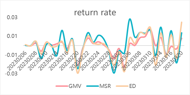
Figure 1: Cumulative Return.

But for Minimum Volatility portfolio, the final return of the portfolio is -0.0679%, which is negative. Therefore, the return performance of Minimum Volatility portfolio is not better than that of the market level, but also not better than that of Maximum Sharpe Ratio portfolio (See Fig. 1).

5. Conclusion

At present, the research on investment portfolio is mostly concentrated in single industry and related industries, while the research on industries with large business scope is lacking. This paper has officially noticed this point, and selected real estate industry, Food and beverage industry, energy industry, medicine industry, finance industry and retail industry in order to inspire and reference other potential investors.

It is found that the financial insurance industry and the food and beverage industry occupy the largest share in the portfolios. However, in the end, when evaluating the performance of these portfolios, the comparison result deviated from the expectation, and the performance of the maximum Sharpe ratio portfolio was the best.

There may also be some areas for improvement in the research process of this article. Firstly, the experiment selected leading enterprises from different industries for configuration, but did not eliminate the differences in industry returns. So, throughout the entire process of calculating weights, the performance of certain stocks has not been strong. Secondly, ARIMA time series analysis also encountered some challenges in determining model parameters, which may be related to the instability of stock data itself.

References

[1]. Markowitz, H.: Portfolio Selection: Efficient Diversification of Investments. Yale University Press (1968).
[2]. Markowitz, H.: Portfolio Selection. Journal of Finance (7), 77 (1952).
[3]. Lin, H., He, J.M.: The Defects of VaR in Portfolio Application and the CVaR Model. Finance & Trade Economics 12), 46 (2003)
[4]. Kang, Z.L., Li, Z.F.: CVaR robust mean-CVaR portfolio optimization model and the solving methods. Operations Research Transactions, 21(1), 1-12 (2017).
[5]. Eftekharian, S. E., Shojafar, M., Shamshirband, S.: 2-phase NSGA II: An optimized reward and risk measurements algorithm in portfolio optimization. Algorithms 10(4), 130 (2017).
[6]. Liu, R.Z., Zhou, Y.: Index Tracking Portfolio and Index Predictability under Multiple Information: Based on Adaptive LASSO and ARIMA-ANN Methods. Systems Engineering (4), 7 (2015).
[7]. Yin, X.G.: Research on Portfolio Selection Based on Machine Learning. China CIO News (12), 4 (2021).
[8]. Zhang, Y.: Stock Price Prediction Based on ARIMA and AT-LSTM Combination Models. Computer Knowledge and Technology (011) (2022).
[9]. Zhang, Z., Zohren, S., Roberts, S.: Deep Learning for Portfolio Optimisation. Papers (2020).
[10]. William, F. Sharpe.: A Simplified Model for Portfolio Analysis. Management Science9(2), (1963).
Cite this article
Yang,W. (2023). Application of ARIMA in Mean-Variance Portfolio Optimization. Advances in Economics, Management and Political Sciences,36,11-16.
Data availability
The datasets used and/or analyzed during the current study will be available from the authors upon reasonable request.
Disclaimer/Publisher's Note
The statements, opinions and data contained in all publications are solely those of the individual author(s) and contributor(s) and not of EWA Publishing and/or the editor(s). EWA Publishing and/or the editor(s) disclaim responsibility for any injury to people or property resulting from any ideas, methods, instructions or products referred to in the content.
About volume
Volume title: Proceedings of the 7th International Conference on Economic Management and Green Development
© 2024 by the author(s). Licensee EWA Publishing, Oxford, UK. This article is an open access article distributed under the terms and
conditions of the Creative Commons Attribution (CC BY) license. Authors who
publish this series agree to the following terms:
1. Authors retain copyright and grant the series right of first publication with the work simultaneously licensed under a Creative Commons
Attribution License that allows others to share the work with an acknowledgment of the work's authorship and initial publication in this
series.
2. Authors are able to enter into separate, additional contractual arrangements for the non-exclusive distribution of the series's published
version of the work (e.g., post it to an institutional repository or publish it in a book), with an acknowledgment of its initial
publication in this series.
3. Authors are permitted and encouraged to post their work online (e.g., in institutional repositories or on their website) prior to and
during the submission process, as it can lead to productive exchanges, as well as earlier and greater citation of published work (See
Open access policy for details).