1. Introduction

Financial investment forecasting and decision-making is a special kind of economic analysis, which plays an extremely important role in improving the level of economic management, improving the accuracy of decision-making and reducing the blindness of decision-making. Decision analysis and outcome prediction are much more difficult in financial investment than in industry or medicine because there is more human activity and human will involved. On the basis of previous studies, some laws in the process of economic development are understood, such as the continuity of economic development and so on [1]. At the same time, all economic phenomena are a process of change over time. For example, a fuzzy stochastic model for real-time predicting of stock prices is proposed [2]. The method of Markov chain is also widely used [3]. As an important part of stochastic process, Markov chain opens up a new way for the analysis and prediction of financial investment, and enriches the content of economic prediction method [4]. From the angle of machine learning, numerous ways have been implemented [5-6].

This paper combines moving average and Markov chain, and seeks to prove that the accuracy of MACD is better than SMA and EMA. Simple moving average (SMA), exponential moving average(EMA), moving average convergence divergence (MACD) are firstly employed to analyze and predict the stock price of Xiaomi Inc from the angle of moving average. Afterwards, this paper analyzes and forecasts the economic trend by using Markov forecast method. The results of two angles are compared and combined.

During the period selected by this paper, both Xiaomi Inc’s developing strategy and the economic environment are stable, highlighting the mathematical rules in the changing of stock price.

2. Simple Moving Average(SMA)

SMA works as follows:

\( SMA({P_{t}},n)=\frac{{P_{t-1}}+{P_{t-2}}+…+{P_{t-n}}}{n} \) (1)

where \( {P_{t}} \) stands for price of an asset at period \( n \) ，and \( n \) stands for number of total periods. Considering the time period of data, 50 days are chosen as long-term moving period, and 20 days as short-term moving period. The historical daily adjust closing price from 2019-01-02 to 2021-12-31 is as below:

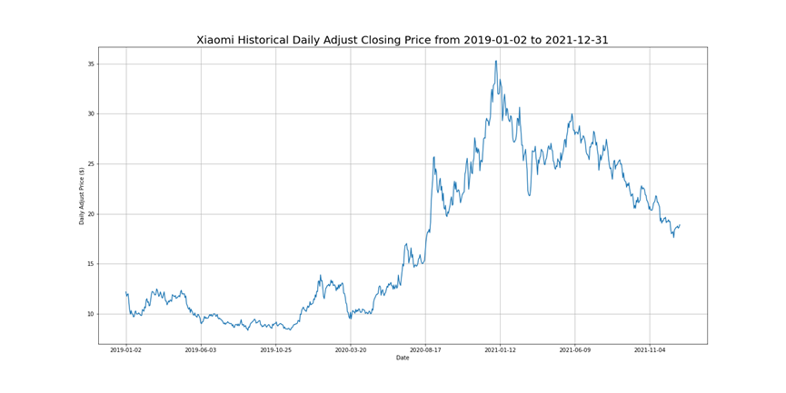
Figure 1: Xiaomi Historical Daily Adjust Closing Price from 2019-01-02 to 2021-12-31.

According to SMA,

\( {r_{t}}=\frac{SMA({P_{t}},s)-SMA({P_{t}},L)}{SMA({P_{t}},L)} \) .(2)

If \( {r_{t}} \) is greater than 0, then the trade signal should be “BUY”. If \( {r_{t}} \) is less than 0, then the trade signal should be “SELL”. In other words, the trade signal should be “BUY” when \( SMA({P_{t}},20) \gt SMA({P_{t}},50) \) , while be “SELL” when \( SMA({P_{t}},20) \lt SMA({P_{t}},50) \) .

The result is as follows:

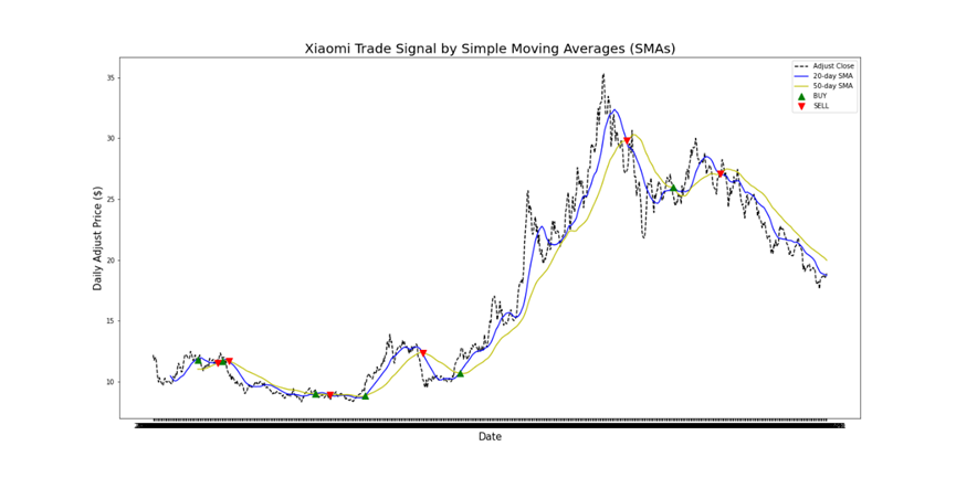
Figure 2: Xiaomi Trade Signal by Simple Moving Averages (SMAs).

In the graph above: Blue line represents the Faster Moving Average (20 day SMA). Yellow Line represents the Slower Moving Average (50 day SMA). Black Line represents the Adjust Closing Price.

Moreover, It shows that the Short-Term (20 day SMA) Moving Average closely resembles the adjust closing price. This can be accounted for it taking into consideration more recent prices. In contrast, the Long-Term (50 day SMA) Moving Average has comparatively more lag and loosely resembles the actual price curve.

\( ∆ \) represents Trade Signal "BUY", it occurs when Faster Moving Average (20 day SMA) crosses above Slower Moving Average(50 day SMA), Which can be understood as the average price over last 20 days has risen above the average price of past 50 days.

\( ∇ \) represents Trade Signal "SELL", it occurs when Faster Moving Average (20 day SMA) crosses below Slower Moving Average (50 day SMA), which can be understood as the average price in last 20 days has fallen below the average price of the last 50 days.

Final Portfolio Value equals to $2.25. Total Return equals to 124.83%. B&H Return equals to 86.91%. Max Drawdown equals to 24.95%. Win Percentage equals to 49.93%.

3. Exponential Moving Average(EMA)

Exponential Moving Average (EMA), which gives more weight to the most recent period, can reduce the lag induced by the use of the SMA. The result of EMA is more reliable than SMAs as it is comparatively a better representation of the recent performance of the asset.

\( EMA({P_{t}},β)=β{P_{t}}+(1-β)EMA({P_{t-1}},β) \) (3)

where \( β=\frac{2}{n+1} \lt 1 \) .

According to EMA,

\( {r_{t}}=\frac{EMA({P_{t}},s)-EMA({P_{t}},L)}{EMA({P_{t}},L)} \) (4)

The result is as follows:

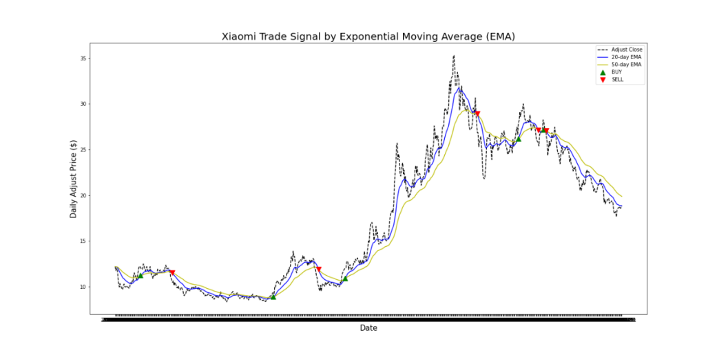
Figure 3: Xiaomi Trade Signal by Exponential Moving Average(EMA).

There are 2 advantages of Exponential Moving Average (EMA) over the Simple Moving Average (SMA):

EMA also includes all the data in the life of instrument. However, it assigns a greater weight to the more recent data. It is a weighted moving average.

User is able to adjust the weighting to give greater or lesser weight to the most recent day’s price, which is added to a percentage of the previous day’s value. The sum of both percentage values adds up to 100.

Final Portfolio Value equals to $2.07. Total Return equals to 107.39%. B&H Return equals to 75.58%. Max Drawdown equals to 33.64%. Win Percentage equals to 49.39%.

4. Moving Average Convergence Divergence (MACD)

On top of SMA and EMA, the relationship between 2 moving averages with different time periods are compared, which is also known as moving average convergence divergence(MACD) [7]. In this model, \( {MACD_{t}}=EMA({P_{t}},12)-EMA({P_{t}},26) \) , and \( Signal Line=EMA({MACD_{t}},9) \) . When \( {MACD_{t}} Line \) cross \( Signal Line \) from below, the signal is buy.

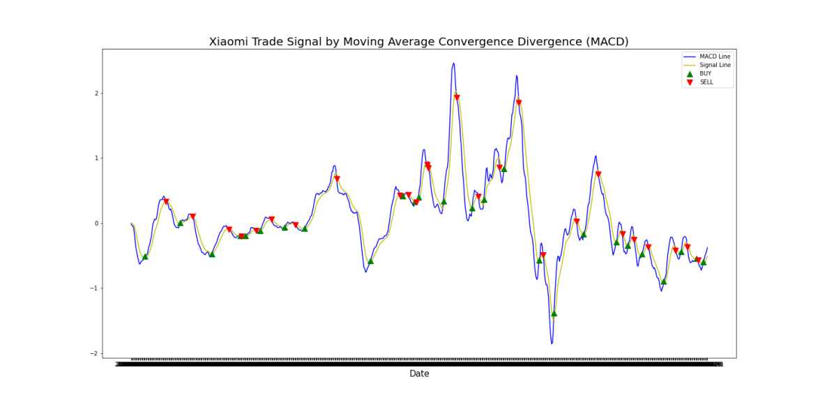
Figure 4: Xiaomi Trade Signal by Moving Average Divergence(MACD).

Final Portfolio Value equals to $4.90. Total Return equals to 390.04%. B&H Return equals to 267.53%. Max Drawdown equals to 5.87%. Win Percentage equals to 52.98%.

5. Markov Chain

Markov chain is a special case of stochastic process, which is first proposed and studied by Russian mathematician Markov, and has formed a complete and rich theory so far. It describes a random process in which, if the state of the system is known at time, the state of the system before time has no effect on what happens after time. In other words, under the condition of known "present", the evolution of process "future" has nothing to do with "past". This is called memorylessness [8].

If the state space of stochastic process \( \lbrace {X_{n}},n=0,1,2,…\rbrace \) is \( E=\lbrace n=0,1,2,…\rbrace \) , then for any given nonnegative integer \( k,l \) and \( 0≤{n_{1}}≤{n_{2}}≤…≤{n_{l}} \lt m \) and \( {i_{{n_{1}}}},{i_{{n_{2}}}},…,{i_{{n_{l}}}},{i_{m}},{i_{m+k}}∈E \) ,

\( P\lbrace X(m+k)={i_{m+k}}丨X(m)={i_{m}},X({n_{l}})={i_{{n_{l}}}},…,X({n_{2}})={i_{{n_{2}}}},X({n_{1}})={i_{{n_{1}}}}\rbrace \)

\( =P\lbrace X(m+k)={i_{m+k}}丨X(m)={i_{m}}\rbrace \) (5)

Then \( \lbrace {X_{n}},n=0,1,2,…\rbrace \) is called Markov chain. Moreover, it satisfies that \( P\lbrace {X_{m+1}}=j丨{X_{m}}=i\rbrace ={p_{ij}} \) , where \( 0≤{p_{ij}}(m)≤1∀i,j∈E \) , and \( \sum {p_{ij}}(m)=1 \) .

The changes of stock price are divided into three kinds of states, which are distinguished by subscripts: up \( {r_{1}} \) , flat \( {r_{2}} \) , down \( {r_{3}} \) . The state space is \( E({x_{1}}, {x_{2}}, {x_{3}}) \) . The probability \( {p_{ij}} \) is denoted as the probability of \( Π(i)=({p_{1}},{p_{2}}, {p_{3}}) \) , which transforms state \( i \) into state \( j \) .

In the selected data set, there are a total of 741 trading days. Among them, there are 318 up, 29 flat, 394 down. Therefore, \( {p_{1}}=\frac{318}{741} \) , \( {p_{2}}=\frac{29}{741} \) , \( {p_{3}}=\frac{394}{741} \) . \( Π(0)=(\frac{318}{741},\frac{29}{741},\frac{394}{741}) \) . According to the data, the total number of rising times is 318, among which there are 120 times when the rising state changes to the rising state, then the transfer probability is \( {p_{11}}=\frac{120}{318} \) ; there are 16 times when the rising state changes to the flat state, then the transfer probability is \( {p_{12}}=\frac{16}{318} \) ; there are 182 times when the rising state changes to the falling state, then the transfer probability is \( {p_{13}}=\frac{182}{318} \) . The same is true for flat state and down state. Therefore, the stock closing state transfer matrix is as follows:

\( P=[\begin{matrix}{p_{11}} & {p_{12}} & {p_{13}} \\ {p_{21}} & {p_{22}} & {p_{23}} \\ {p_{31}} & {p_{32}} & {p_{33}} \\ \end{matrix}]=[\begin{matrix}\frac{120}{318} & \frac{16}{318} & \frac{182}{318} \\ \frac{16}{29} & 0 & \frac{13}{29} \\ \frac{182}{393} & \frac{13}{393} & \frac{198}{393} \\ \end{matrix}] \) (6)

Since the first data is down, the denominator of \( {p_{31}},{p_{32}},{p_{33}} \) is 393 rather than 394. According to Markov chain, the state probabilities of different periods are expressed by the state vector \( Π(i) \) , which satisfies that \( Π(i)=Π(i-1)P \) . The stationary distribution is \( Π=(\frac{159}{370},\frac{29}{740},\frac{393}{740}) \) , which represents that after enough time, the probability of stock price rising is \( \frac{159}{370} \) , the probability of stock price remaining flat is \( \frac{29}{740} \) , the probability of stock price dropping is \( \frac{393}{740} \) .

Then the data are divided into three parts according to the closing price. Among all the data, the lowest closing price is $8.35, while the highest closing price is $35.3. The division is as follows: (1) lower than $17, (2) higher than $17 but lower than $26, (3) higher than $26. Similarly, the Markov chain can eb established, and the stock closing price transfer matrix can be solved:

\( P=[\begin{matrix}{p_{11}} & {p_{12}} & {p_{13}} \\ {p_{21}} & {p_{22}} & {p_{23}} \\ {p_{31}} & {p_{32}} & {p_{33}} \\ \end{matrix}]=[\begin{matrix}\frac{398}{400} & \frac{2}{400} & 0 \\ \frac{1}{210} & \frac{199}{210} & \frac{10}{210} \\ 0 & \frac{10}{130} & \frac{120}{130} \\ \end{matrix}] \) (7)

According to Markov chain, the stationary distribution is \( Π=(\frac{10}{27},\frac{7}{18},\frac{13}{54}) \) , which represents that after enough time, the probability of stock price lying in the ($8.35, $17) is \( \frac{10}{27} \) , the probability of stock price lying in range ($17, $26) is \( \frac{7}{18} \) , the probability of stock price lying in the ($26, $35.3) is \( \frac{13}{54} \) .

6. Conclusion

On one hand, among SMA, EMA and MACD, their win percentages are similar, but MACD has the lowest max drawback and the highest total return. Therefore, the accuracy of MACD is better than SMA and EMA on the prediction of Xiaomi stock data from January 2, 2019 to December 31, 2021.

On the other hand, from the angle of Markov chain, there are two ways of dividing the data: price changing state, and closing price. Since most of the price changing states are down, the stationary distribution of the selected data shows that the stable probability of stock price change is most likely to go down. However, if the value is taken into account and the data are analyzed using the second Markov chain, the results are more accurate and fit with conclusion from methods of moving average.

There are various other methods to analyze and forecast stock price, where moving average and Markov process are solely part of this field. Therefore, more research can be done based on the results of this paper and intersection with others.

References

[1]. Yuanlie Lin. (2002). Applied Stochastic Processes. Tsinghua University Press.
[2]. Wang Y F. On-demand forecasting of stock prices using a real-time predictor[J]. IEEE Transactions on Knowledge and Data Engineering, 2003, 15(4): 1033-1037.
[3]. Choji D N, Eduno S N, Kassem G T. Markov chain model application on share price movement in stock market[J]. Computer Engineering and Intelligent Systems, 2013, 4(10): 84-95.
[4]. Long Yan, Cong Lin, Jiahui Zhu. Application of Markov chain in financial investment [J]. Journal of Ningbo Institute of Technology,2017,29(04):1-8.
[5]. Chowdhury R, Mahdy M R C, Alam T N, et al. Predicting the stock price of frontier markets using machine learning and modified Black–Scholes Option pricing model[J]. Physica A: Statistical Mechanics and its Applications, 2020, 555: 124444.
[6]. Leung C K S, MacKinnon R K, Wang Y. A machine learning approach for stock price prediction[C]//Proceedings of the 18th International Database Engineering & Applications Symposium. 2014: 274-277.
[7]. Yongjie Yang. Prediction Method of Stock price Change Trend Based on Optimized MACD Model [J]. Journal of Guangxi Academy of Sciences,2017,33(1):65-70
[8]. Cihua Liu. Stochastic Process [M]. Wuhan: Huazhong University of Science and Technology Press, 2001:20-35.
Cite this article
Qian,H. (2023). Stock Price Prediction: Moving Average and Markov Chain. Advances in Economics, Management and Political Sciences,36,66-71.
Data availability
The datasets used and/or analyzed during the current study will be available from the authors upon reasonable request.
Disclaimer/Publisher's Note
The statements, opinions and data contained in all publications are solely those of the individual author(s) and contributor(s) and not of EWA Publishing and/or the editor(s). EWA Publishing and/or the editor(s) disclaim responsibility for any injury to people or property resulting from any ideas, methods, instructions or products referred to in the content.
About volume
Volume title: Proceedings of the 7th International Conference on Economic Management and Green Development
© 2024 by the author(s). Licensee EWA Publishing, Oxford, UK. This article is an open access article distributed under the terms and
conditions of the Creative Commons Attribution (CC BY) license. Authors who
publish this series agree to the following terms:
1. Authors retain copyright and grant the series right of first publication with the work simultaneously licensed under a Creative Commons
Attribution License that allows others to share the work with an acknowledgment of the work's authorship and initial publication in this
series.
2. Authors are able to enter into separate, additional contractual arrangements for the non-exclusive distribution of the series's published
version of the work (e.g., post it to an institutional repository or publish it in a book), with an acknowledgment of its initial
publication in this series.
3. Authors are permitted and encouraged to post their work online (e.g., in institutional repositories or on their website) prior to and
during the submission process, as it can lead to productive exchanges, as well as earlier and greater citation of published work (See
Open access policy for details).