1. Introduction

Among all the marketing practices, it is important to have a specific prediction of the future sales. Which can lead the organizations or companies allocate the suitable resources to its various departments to prepare for the future sales.

The accuracy of the prediction of future sales affects a lot to the business outcomes. And as the markets nowadays are becoming more and more complex and changeable, the task of prediction becomes more complicated. So, this research must research or learn more about the process of business analysis to improve the theory about increasing the accuracy of sales prediction.

There are a lot of research here talking about the sales prediction and give us a number of inspirations containing create different kinds of models, creation of new variables, new methods of finding the relations of different variables and so on. Here are some related research that gives this article some experience about the business prediction, covering Bayesian estimation of the generalized bass model [1], regression model for predicting weather impact on high-volume low-margin retail products [2], periodic grey model for automobile prediction [3], censored demand prediction by machine learning [4], sales predictive algorithms base on ANN [5], for Andres’ study, Bass model-based Bayesian estimation model, Andres proposed a Bayesian estimation of the general Bass model to predict product sales based on historical data of single product or similar products (pre-launch forecast), from this research, it achieves the prediction for new product without any historical sales data by analogy. Gylian in his article set a connection between the long-term forecasting model and the short-term forecasting model. Lixiong Gong in his research improves the linear regression model to achieve the prediction to the nonlinear problems, which all give this research a lot of insights.

But the current research still exist some problems, sometimes they face Inaccurate peak prediction due to neglect of peak-to-peak interactions, current research still doesn’t know how to capture appropriate influencing factors as model input. And about the models’ descriptions there still need more studies.

As there still have these kinds of problems this research mentioned above, this research analyzes the process of big mart’s sales prediction to organize the whole logic of prediction through historical data. This research first downloads the dataset of big mart, did data cleaning and organizes its variables’ distributions. Then the research does some feature engineering practices and selects some important features. Finally, it creates five simple models to predict the outlet-sales and use the MAR measure to measure each models’ performances.

2. Data Description

The big mart data set is collected by scientists in mart for 1559 products among 10 various stores in different cities.

The dataset has 11 columns and 11 fields, founded 2 years ago. And it should be noted that data may have missing values, as some stores may not report all data due to some practical problems.

The data set provides product details and output information for purchased products with their selling value divided into a train set (8523) and a test set (5681) (See Table 1).

Table 1: Some information about the datasets.

3. Correlation Matrix

A correlation matrix is just an array that shows the correlation coefficients for various variables. The matrix puts the relationship among all possible value pairs into an array. It is a useful and important tool for summarizing an extensive dataset and for identifying and visualizing patterns in the data [6].

Correlation matrix plays a very important role in analyzing various different variables’ relationship and classifying the connections between all these variables. A correlation matrix is a chart or an array. This research can simply apply a correlation table in excel. And the coefficient between these two variables can be applied for the latter analysis.

4. Feature Selection

The feature selection methods contain two types: Filter type, Wrapper type.

4.1. Filter

For Filter method, as its name shown, it is more like a filter that this research put all the valuable features into the filter machine, this research set specific criteria for the filter, finally this research gets the appropriate features this research need.

Based on the attributes of the features, such as feature variance and feature relevance to the response, the filter type feature selection method assigns a value to each feature's importance. As part of a data preprocessing procedure, you choose significant features, and then you train a model using those chosen features [7].

In this article, this research uses a specific filter method called KS & Churn Detection Rate Univariate Filter. This research set criteria that the features whose KS score and CDR score above 0.1 should be selected.

4.2. Wrapper

For the wrapper method, it just combines different variables into different sets and check which sets’ accuracy is the highest. Then select the most appropriate set.

A selection criterion is used by the wrapper type feature selection method to add or delete features once training is completed using a subset of features. The addition or removal of a feature alters the performance of the model, and this is directly measured by the selection criterion. A model is trained and improved repeatedly by the algorithm until its halting requirements are met [7].

In this article, this research will use Stepwise selection wrapper. There are two types of stepwise selection methods: one is called forward stepwise selection and the other is backward stepwise selection.

For the forward stepwise selection, this research just puts the variables one by one into the set and calculates the accuracy, every time this research put in the variables, this research selects the highest accuracy variables. Finally, will get all the features this research wants.

For the backward stepwise selection, the process is as similar as the forward stepwise selection, but this research just picks all the features in and eliminates the features on by one, calculate the accuracy and pick the best set.

5. EDA

EDA’s full name: explore data analysis. The author classifies each item’s amount, percentage, mean standard and others to gain the distribution of each single item’s property.

After some basic data operating, the author gains the outcome of each item (See Fig. 1 and Fig. 2).

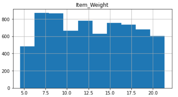
Figure 1: Item-weight distribution.

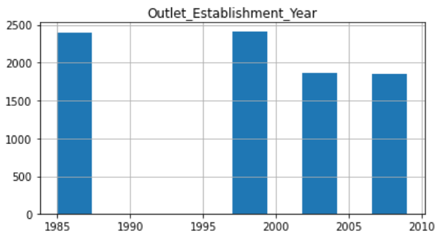
Figure 2: Establishment year distribution.

Here are some examples of the item’s distribution.

From the above Fig. 1 and Fig. 2, the amounts of customers attaining the highest when the item weight are between 7 and 9 units. And every kind of different weighted product can be acceptable by customers, that seems the weight of product affect not that much to the customer’s decisions.

For the Outlet establishment year, that distribution seems not that normal, people are willing to buy the product established in 1985 or in 1999. And product established during 1990 to 1997 seems not that acceptable by customers.

Other to the distributions, for this case, the author will do some basic plots showing the relations between different variables. the plots under just shows the relations between MRP and the outlet sales (See Fig. 3).

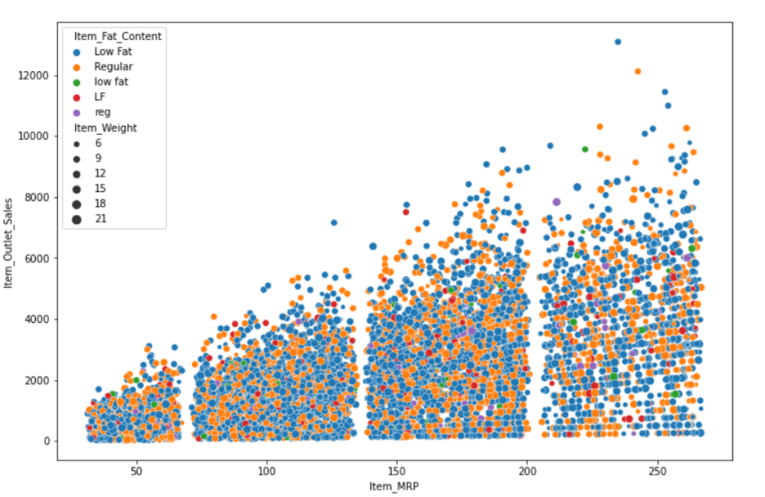
Figure 3: MRP and outlet-sales plot.

6. Feature Engineering

As to the process of feature engineering, firstly the author applies correlation matrix to the various variables, then find the connection between different properties and the degree of relations (See Fig. 4).

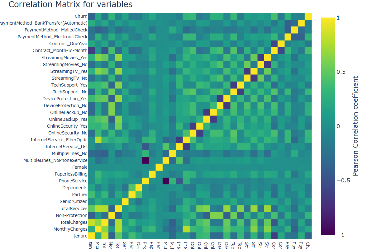
Figure 4: Correlation matrix.

For this case, this research does not have such many features and the matrix will be not that complex.

7. Feature Selection

The process of Feature selection is an important part in this article, through the process of feature selection, finally this research will find which factor of product mostly affect people’s decisions to choose.

By means of the use of only a portion of the measured characteristics (predictor variables), Feature selection diminishes data dimensionality. Subject to limitations such as necessary or excluded characteristics and subset size, feature selection algorithms seek a subset of predictors that model the best observed responses. Better predictive performance, faster and cheaper predictors are the main benefits of choosing features. Even when all features are relevant and provide information on response variables, the use of too many features can reduce forecast performance [7].

When applying the feature selection method, this research should be careful, as when this research eliminates an important feature, this research lose accuracy. But if this research adds an unrelated feature, this research cost a lot to predict the outcome.

7.1. KS & Churn Detection Rate Univariate Filter

KS & Churn Detection Rate Univariate Filter is a kind of filter method this research has talked above, for this process, the author just collects the KS score and other scores and then calculate the average. Using the special algorithm, the author sets a standard for the features’ scores then finally gets the features this research wants.

An example of this kind of method’s outcomes just like this in Table 2.

Table 2: Results of KS & Churn Detection Rate Univariate Filter.

7.2. Stepwise Selection Wrapper

Then, after doing the filter process, the author applies the stepwise selection wrapper to the selected features. Using the machine learning algorithm, the author calculates different feature’s sets and select the most suitable set that have the highest accuracy.

Then after doing all the process of feature selection, this research still has to test if our outcomes or our methods are correct.

This research distributes the total data into two sets, one train data and test data, this research use train data to apply the methods to it and create the model, and this research use the test data to calculate the accuracy and determine whether the outcome is correct.

7.3. Testing Data

Once you have built your machine learning model (based on your training data), you have to find invisible data to test your model. These data are called test data, you have the right to take use of them to measure the performance of the models and progression of the training of your mathematical process and adjust or optimize it to improve the outcomes [8].

8. Modeling

Machine learning models are the backbone of innovation in all areas of retail funding.

Machine learning models are foundational in all areas, from fundamental science to marketing, funding, retail and more. Nowadays, few industries are sheltered from the machine learning revolution, which has changed not only the way businesses operate, but its total development process.

Machine learning models are created based on the machine learning foundations, which are formed with tagged, unlabeled or blended data. Every kind of machine learning algorithm is tailored for its own specific purpose, such as recognition or predictive modelling, so that data scientists use special needed algorithms as the basis for different models. When data is captured by a special mathematical process, it is modified to better handle a specific task and becomes a machine learning model [9,10].

As to the modeling, finally the author implements 5 models: linear regression model, Random Forest Regressor model, K Neighbors Regressor model, Gradient Boosting Regressor model, XGB Regressor model.

Using the MAE standard to measure the performance of the models, finally will find the final suitable model for prediction of the outlet-sales (See Table 3).

Table 3: Model Comparison.

As MAE is the mean absolute error, the most suitable model should be the lowest value. So, the XGB Regressor model is the most suitable one.

9. Conclusion

After doing all this machine learning methods and operations to analyze the big mart data. The feature that affects customers’ decisions most is the Outlet Type Grocery Store. The big mart and single outlet owners should focus on the type of the grocery more. Item MRP is a significant factor that affect the amounts of sales, it is easy to understand as customers cares the price of the product more. Outlet years also can be seen as an important factor to affect customers’ decisions. What’s more, when predicting the outlet sales, XGB Regressor are recognized as the most suitable one from this article using MAE standard to measure the performance of the models.

References

[1]. Ramírez-Hassan, A., Montoya-Blandón, S.: Forecasting from others’ experience: Bayesian estimation of the generalized Bass model. International Journal of Forecasting 36(2), 442-465 (2020).
[2]. Verstraete, G., Aghezzaf, E. H., Desmet, B.: A data-driven framework for predicting weather impact on high-volume low-margin retail products. Journal of Retailing and Consumer Services 48, 169-177 (2019).
[3]. Gong, L., Wang, C.: Model of Automobile Parts Sale Prediction Based on Nonlinear Periodic Gray GM (1, 1) and Empirical Research. Mathematical Problems in Engineering (2019).
[4]. Ozhegov, E. M., Teterina, D.: Methods of machine learning for censored demand prediction. In Machine Learning, Optimization, and Data Science: 4th International Conference, 441-446 (2019).
[5]. Massaro, A., Maritati, V., Galiano, A.: Data Mining model performance of sales predictive algorithms based on RapidMiner workflows. International Journal of Computer Science & Information Technology 10(3), 39-56 (2018).
[6]. Correlation matrix. Corporate Finance Institute. (2023, March 24). i. https://corporatefinanceinstitute.com/resources/excel/correlation-matrix/,last accessed 2023/7/5
[7]. Rankfeatures. MathWorks. (n.d.). https://www.mathworks.com/help/stats/feature-selection.html, last accessed 2023/7/5
[8]. The difference between training data vs. test data in machine learning. Data Science without Code(2022,February 11), https://www.obviously.ai/post/, last accessed 2023/7/5.
[9]. Machine learning models: What they are and how to build them. Coursera.(n.d.). i. https://www.coursera.org/articles/machine-learning-models last accessed 2023/7/5.
[10]. Bevans, R. (2022, November 15). Simple linear regression: An easy introduction & examples. Scribbr. https://www.scribbr.com/statistics/simple-linear-regression/last accessed 2023/7/5.
Cite this article
Zhao,Z. (2023). Research on the Distributions of Products for Big Mart. Advances in Economics, Management and Political Sciences,43,32-39.
Data availability
The datasets used and/or analyzed during the current study will be available from the authors upon reasonable request.
Disclaimer/Publisher's Note
The statements, opinions and data contained in all publications are solely those of the individual author(s) and contributor(s) and not of EWA Publishing and/or the editor(s). EWA Publishing and/or the editor(s) disclaim responsibility for any injury to people or property resulting from any ideas, methods, instructions or products referred to in the content.
About volume
Volume title: Proceedings of the 7th International Conference on Economic Management and Green Development
© 2024 by the author(s). Licensee EWA Publishing, Oxford, UK. This article is an open access article distributed under the terms and
conditions of the Creative Commons Attribution (CC BY) license. Authors who
publish this series agree to the following terms:
1. Authors retain copyright and grant the series right of first publication with the work simultaneously licensed under a Creative Commons
Attribution License that allows others to share the work with an acknowledgment of the work's authorship and initial publication in this
series.
2. Authors are able to enter into separate, additional contractual arrangements for the non-exclusive distribution of the series's published
version of the work (e.g., post it to an institutional repository or publish it in a book), with an acknowledgment of its initial
publication in this series.
3. Authors are permitted and encouraged to post their work online (e.g., in institutional repositories or on their website) prior to and
during the submission process, as it can lead to productive exchanges, as well as earlier and greater citation of published work (See
Open access policy for details).