1. Introduction

Stock investment is one of the main means of investment. For investors, choosing which stocks will reduce the risk of loss and provide a decent return when faced with thousands of stocks requires some help [1]. With the advent of AI (artificial intelligence) research results, it is possible to bring AI-related research into stock prediction.

The stock market produces a large amount of trading data every day, which often hides a large amount of useful information. Excavating useful information from these data and predicting the future trend of stock prices can help investors and securities institutions make scientific investment decisions and reduce investment risks [2].

Stock price prediction model can be divided into traditional model, machine learning model and deep learning model. Traditional regression models, such as ARIMA model, GARCH model. Such models usually require the time series to have the characteristics of stationarity, which conflicts with the nonlinear, highly complex and non-stationarity characteristics of the stock market. With the rise of big data, machine learning and other technologies, a variety of machine learning models are more suitable for the relevant needs of financial market time series research [3]. Machine learning models can capture internal relationships that are difficult to be found. Common machine learning models for stock prediction include support vector machine, random forest, K proximity value, etc [4].

In recent years, many scholars forecast stock price trend through machine learning model combining stock market characteristics, company characteristics, transaction characteristics and so on. A large number of empirical studies also show that machine learning plays a significant role in stock price trend prediction.

For example, Phua et al. conducted a study to predict the trend of five major stock indexes with a prediction accuracy higher than 60% by building a neural network model [5]. Oztekin et al. proved that support vector machine (SVM) has significant predictive ability even in terms of out-of-sample performance, and compared the predictive ability of SVM model, MLP-based neural network model and Adaptive Network-based Fuzzy Inference System (ANFIS), among which SVM has the best performance [6]. Kim trained the SVM model with the daily time series of the Korean stock market, and the successful rate of the model was about 56% [7].

In general, it is very difficult to predict the true price of a stock and relatively easy to predict the rise and fall of a stock price. In this paper, the aim of the prediction is just to determine the rise and fall.

Random forest can effectively run on large data sets with high accuracy and good anti-noise ability. Randomness is introduced in the model so it is not easy to overfit [8]. Logistic regression is very easy to implement and efficient to train. So it is also a good benchmark against which to measure the performance of other more complex algorithms [9]. Svm supports solving binary classification, which can train small sample models with strong generalization ability to deal with high dimensional problems and deal with interaction of nonlinear features with kernel function [10]. These models all have a range of advantages, so they are selected to be used in this paper.

The data is collected from Tushare interface first, and then performs data cleaning and preprocessing. Since there are many stock market change factors, the relevant feathers are extracted from the daily trading data. These feathers are input into each specific algorithm after gaining the relevant data set. Finally, the experimental results of three models are compared and analyzed in detail by using some indicators and figures.

The remainder of this organized as follows: In Section 2, the methodologies of three models are introduced firstly. In the following Section 3, the experimental study is operated in python to apply three methodologies. The structure of Section 3 is: Data collection-Feature extraction-Model establishment-Result analysis. In Section 4, the results gained in Section3 are shown in line graph to compare three models clearly. Finally, the results are concluded.

2. Methodology

2.1. Random Forest

Random forest is a machine learning algorithm based on decision tree. Its basic unit is the decision tree. The number of decision trees and the input characteristics of a single decision tree are the two main parameters in the method. Classification and regression issues can both be solved using the random forest approach. Before modeling, Bootstrap sampling method was adopted for the data. Random extraction method with place back was adopted to extract one sample each time from n samples for a total of n times, forming a training sample with a sample size of n. Then, some features were randomly selected from the sample for the establishment of decision trees, and a big amount of decision trees were established through repeated sampling and training steps, thus forming a random forest.

According to the algorithm, the algorithm is to construct multiple decision trees and each decision tree will output a value or category. For classification problems, voting is adopted, that is, the principle of minority obedience to majority is adopted to make decisions. The main steps of the algorithm are as follows [11]:

Input:

1. Original train set \( S=\lbrace ({x_{i}},{y_{i}}),i=1,2,⋯,n\rbrace ,(X,Y)∈{R^{d}}×R; \)

2. The sample to be tested \( {x_{t}}∈{R^{d}} \) ;

(1) Conduct Boostrap sampling on the original training set S. Which means full sampling with put back, then generate training set \( {S_{i}} \) for several times;

(2) A regression model is established for each subsample set to generate a tree without pruning \( \lbrace h(θ,{X_{i}}),i=1,2,⋯,k\rbrace \) ;

a:Randomly select \( {M_{tree}} \) features from all attribute features;

b:On each node, the best features are selected from \( {M_{tree}} \) features according to the minimum mean square error principle;

c:Divide until the tree grows to its maximum size.

Output:

1. Set of trees \( \lbrace {h_{t}},i=1,2,⋯,{N_{tree}}\rbrace \) ;

2. For the sample \( {x_{t}} \) , the regression tree \( {h_{i}} \) outputs \( {h_{i}}({x_{t}}) \) .The final output of random forest algorithm on classification problems is as follows:

\( f({x_{t}})=majority vote\lbrace ({h_{i}}({x_{t}}))\rbrace _{i=1}^{{N_{tree}}} \) (1)

2.2. Logistic Regression

This algorithm is generally used to solve dichotomous problems. Nature of classification is to find a decision boundary in the space to solve the classification of decision. Linear regression plays an important role in predicting continuous values, but can’t complete the classification problem.

For arbitrary test variables \( {X_{i}} \) , \( f({X_{i}}) \) can be labelled by its plus or minus characteristic [12].

Define the follow jump function φ(z):

\( φ(z)=\begin{cases} \begin{array}{c} 0,z \lt 0 \\ 0.5,z=0 \\ 1, z \gt 0 \end{array} \end{cases} \) (2)

Among them, the logical function is specified as sigmoid function, which can map variables to [0,1]. the formula of S-shaped function is:

\( φ(z)=\frac{1}{1+{e^{-z}}} \) (3)

The figure of sigmoid function is shown as Fig. 1:

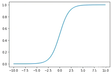
Figure 1: Sigmoid function.

The horizontal axis of is the value of z and the vertical axis represents the function value of the jump function φ(z).

2.3. Support Vector Machine

Support vector Machine (SVM) is a mathematical model based on statistics, which can be used for classification and regression. Like most machine learning classification models, support vector machines are built through training. For linearly indivisible problems, SVM can map training data from linearly indivisible feature space to one. In a higher dimensional space, data that is linearly indivisible can be classified through such a hyperplane. Therefore, the goal of SVM training process is to find an optimal hyperplane.

Given a labeled training dataset:

\( ({x_{1}},{y_{1}}),⋯({x_{n}},{y_{n}}),{x_{i}}ϵ{R^{d}}and {y^{i}}ϵ(-1,1) \) (4)

where \( {x_{i}} \) represents the input variable, \( {y_{i}} \) represents the corresponding classification result. The objective of SVM is to find an optimal hyperplane in the sample space based on the training set D. For the optimization problem to be solved, the hyperplane expression of the function x can generally be expressed by the linear equation (4):

\( w{x^{T}}+ b=0 \) (5)

where w is the coefficient, b is the intercept r, x is the input feature vector.

For all components of the training set, the w and b would meet the following inequalities:

(6)

\( wx_{i}^{T} + b ≤ -1 if yi=–1 \) (7)

Finding the w and b for the hyperplane to segregate the data and maximize the margin \( 1 / {|| w ||^{2}} \) is the goal of training an SVM model.

Vectors \( {x_{i}} \) for which \( |yi| (wx_{i}^{T} + b)= 1 \) will be termed support vector.(See Figure 2.)

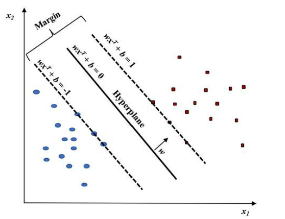
Figure 2: Linear SVM model.

Not all data given in practical problems are linearly separable, some data may be non-linear separable. When there are a lot of characteristic variables, it's complicated to compute the inner product in a higher dimensional space. A kernel function can be used to increase the raw data's dimensionality in a non-linear situation. In a nutshell, a kernel function can speed up some computations that would otherwise require high-dimensional space.

It is defined as:

\( K (x, y)=φ(x)φ(y) \) (8)

Here K is the kernel function. Common kernel functions include Linear kernel, RBF kernel and so on. x, y are n dimensional inputs. \( φ \) is used to map the input from n dimensional to m dimensional space. \( φ(x)φ(y) \) denotes the inner product [13].

3. Model Establishment

3.1. Data Collection

The paper analyzes the stock data of Maotai Company from 2000 to 2022, including seven characteristics. The data is from the tushare package(https://www.tushare.pro/). The raw data contains 5107 rows and 7 columns: the trading date of the stock is listed first, the open price is listed second, the close price is listed third, the daily highest price is listed fourth, the daily lowest price is listed fifth, the number of shares traded is listed sixth, and the stock code is listed seventh.

Data should be pre-processed first. The pandas and numpy will be used to discard the overall missing feature data.

3.2. Feature Extraction

Take a consecutive week closing price for as feather input. There are 7 inputs in this model. Use sklearn. Preprocessing. Scale function in preprocessing module to standardize the feather data.

Take the sign of the daily close price change rate as the forecast target: If the sign of the change rate is negative, then define the label is -1; if the sign of the change rate is positive, then define the label is 1.

3.3. Model Establishment

The data is split into a training set and a test set after finishing data preprocessing and feature extraction. The sample data before January 1, 2022 is set as a training set, a total of 4858 days; the sample data from January 1, 2022 to December 31, 2022 is set as a test data, a total of 242 days’ data. Then the training set is input into the model for training and generate parameters.

Table 1. demonstrates the main parameters of the random forest model:

Table 1: The main parameters.

Table 2. presents the main parameters of the logistic regression model:

Table 2: The main parameters.

Table 3. shows the main parameters of the support vector machine model:

Table 3: The main parameters.

3.4. Model Evaluation

In order to accurately assess the model's forecasting performance, Mean Square Error (MSE) and determination coefficient \( {R^{2}} \) are selected as the evaluation indexes of the model performance. The expression is as follows:

\( MSE=\frac{1}{N}\sum _{i=1}^{N}{({y_{i}}-{\hat{y}_{i}})^{2}} \) (9)

\( {R^{2}}=1-\frac{\sum _{i=1}^{N}{({y_{i}}-{\hat{y}_{i}})^{2}}}{\sum _{i=1}^{N}{({y_{i}}-{\bar{y}_{i}})^{2}}} \) (10)

In the formula \( {y_{i}} \) is the true value; \( {\hat{y}_{i}} \) is the predicted number; \( {\bar{y}_{i}} \) is the average value of test set; N is the number of samples; MSE represents the overall reliability of the forecast data. The prediction findings are more dependable with the lower the MSE and higher R². The MSE is positively correlated with the prediction error, which show the reliability of the prediction results. R² is between 0 and 1, which denotes the degree of fitting between the predicted value and the test set. The better the fitting degree is, the better the prediction performance is, and the closer it is to 1, the better the prediction effect is [14]. The evaluation scores are shown in Table 4.:

Table 4: The evaluation scores.

Besides, other evaluation indicators are run in the python. Model.score function in sklearn is to evaluate the accuracy score of classification. Correct_num function is to calculate the number of results in test set is predicted correctly. The evaluation indicators are shown in Table 5.:

Table 5: The evaluation scores.

4. Comparison Analysis

Because all the results gained are numbers 1 and -1, the numbers are added together to observe the difference between the forecasting values and the real numbers. To compare the predicted results clearly, line charts show the difference between the test value and predicted value. The horizontal axis is the trade date and the vertical axis represents the added value of predicted results “1” and “-1”. The red line represents the predicted result and the bule line show the real test set trend.

Three line charts (Figure 3) are shown below:

Figure 3: Line figure of random forest model.

In random forest model (see Figure 3.), this line graph demonstrates the real test price trend and the predicted trend. The prediction trend totally different from the fact.

Figure. 4: Line figure of logistic regression model.

In logistic regression model (see Figure 4.), the predicted line and the real line almost have the same trend.

Figure. 5: Line figure of svm model.

In the svm model (see Figure 5.), the predicted line has different trend compared with the test set.

It is obvious that logistic regression model fits the data well and the other two models behave poor by observing the line charts. Also, the evaluation scores and indicators also show that logistic regression behave best. It has the smallest RMSE and the biggest R2 among three models. And the accuracy score and correct number of logistic regression model are higher than other two with 0.929 and 255 respectively.

5. Conclusion

In this paper, the random forest, logistic regression and support vector machine are used as the stock trend prediction model in order to predict future rise and fall of stocks. First, select stock data from tushare. After data processing and feather extraction, the original data set was divided into two parts: training set and test set. The training set is used for the real training process and the test set is used to verify the effect of the prediction model. Finally, the model scores are calculated to evaluate the model. Using the evaluation scores and figures to compare, logistic regression model is relatively good in predicting stock problems, which provide new ideas for future stock investment. In feather extraction, this paper only considers the impact of historical data but neglect other important external information, like financial statement and company announcements. More work needs to do to extract the external information and quantize it to feather input.

References

[1]. Xiong,Z.,Che,W.G.: Application of ARIMA-GARCH-M model in short-term stock forecasting. Journal of Shaanxi Technology University (Natural Science Edition)38(04),69-74(2022).
[2]. Zhang, J.K.,Sheng,Y.P.: Support vector machine prediction of stock price rise and fall. Journal of Information Science and Technology University of Beijing (Natural Science) 32(03):41-44.DOI:10.16508/j.cnki.11-5866/n.2017.03.008(2017).
[3]. Liu,Z.S.: Research on stock trend prediction based on Machine learning. UESTC (University of Electronic Science and Technology of China).DOI:10. 27005/d.cnk i.gdzku. 2020.003227(2020).
[4]. Cheng,M.F.,Gao,S.P.: Multi-scale stock forecasting based on deep transfer learning. Computer engineering and applications58(12),249-259(2022).
[5]. Phua, P. K. H., Zhu, X., & Koh, C. H.: Forecasting Stock Index Increments Using Neural Networks with Trust Region Methods.IEEE1,260-265(2003).
[6]. Oztekin, A., Kizilaslan, R., Freund, S., & Iseri, A.: A Data Analytic Approach to Forecasting Daily Stock Returns in an Emerging Market. European Journal of Operational Research253(3),697-710(2016).
[7]. Kim,K J.: Financial Time Series Forecasting Using Support Vector Machines. Neurocomputing55(1),307-319(2003).
[8]. Biau, G., & Scornet, E.: A random forest guided tour. Test,25, 197-227(2016).
[9]. LaValley, M. P.: Logistic regression. Circulation117(18), 2395-2399(2008).
[10]. Chauhan, V. K., Dahiya, K., & Sharma, A.: Problem formulations and solvers in linear SVM: a review. Artificial Intelligence Review52(2), 803-855(2019).
[11]. Cui, X.H.,Liu,C.J., Xue,L.: Prediction of porosity based on stochastic forest regression algorithm. Exploration engineering in western China31(11):99-102+105(2019).
[12]. Jiang,X.L.,Wang,J.H.: Use logical regression model to predict the pathogenic factors of cervical cancer. Computer and information technology30(04):30-32.DOI:10.19414/j.cnki.10 05-1228.2022.04.017(2022).
[13]. Huang, S., Cai, N., Pacheco, P. P., Narrandes, S., Wang, Y., & Xu, W.:Applications of support vector machine (SVM) learning in cancer genomics. Cancer genomics & proteomics15(1), 41-51(2018).
[14]. Fang,Y.H.,Chen,X.W..: Comparative study on estuary salinity prediction based on neural network and support vector machine.Hydrology42(05):51-55.DOI:10.19797/j.cnki.1000-0852.20210194(2022).
Cite this article
Guo,J. (2023). Predict Stock Price Trend by Using Classification Model. Advances in Economics, Management and Political Sciences,45,70-78.
Data availability
The datasets used and/or analyzed during the current study will be available from the authors upon reasonable request.
Disclaimer/Publisher's Note
The statements, opinions and data contained in all publications are solely those of the individual author(s) and contributor(s) and not of EWA Publishing and/or the editor(s). EWA Publishing and/or the editor(s) disclaim responsibility for any injury to people or property resulting from any ideas, methods, instructions or products referred to in the content.
About volume
Volume title: Proceedings of the 2nd International Conference on Financial Technology and Business Analysis
© 2024 by the author(s). Licensee EWA Publishing, Oxford, UK. This article is an open access article distributed under the terms and
conditions of the Creative Commons Attribution (CC BY) license. Authors who
publish this series agree to the following terms:
1. Authors retain copyright and grant the series right of first publication with the work simultaneously licensed under a Creative Commons
Attribution License that allows others to share the work with an acknowledgment of the work's authorship and initial publication in this
series.
2. Authors are able to enter into separate, additional contractual arrangements for the non-exclusive distribution of the series's published
version of the work (e.g., post it to an institutional repository or publish it in a book), with an acknowledgment of its initial
publication in this series.
3. Authors are permitted and encouraged to post their work online (e.g., in institutional repositories or on their website) prior to and
during the submission process, as it can lead to productive exchanges, as well as earlier and greater citation of published work (See
Open access policy for details).