1.Introduction

1.1.Research Background and Significance

Crude oil price plays a vital role in oil-importing countries like the United States, particularly in the transportation and manufacturing sectors [1]. For the U.S., the breakeven inflation rate is closely linked to oil prices for most of the period. An oil price increase can lead to inflation and higher interest rates [2]. In specific, the causality-in-variance between WTI crude oil price and inflation is significant in both directions, implying the predictive power of crude oil price for CPI [3]. Therefore, it is plausible to predict U.S. inflation based on crude oil prices.

Inflation prediction has been a major interest because it sheds light on decision makings. Given the significant link between unemployment and inflation, governments, central banks, and policymakers rely on the prediction to enact monetary and fiscal policies, set interest rates, and manage stability [4]. In the context of the Russia-Ukraine conflict, according to The Federal Reserve, the rising commodity prices and oil prices imposed a downward pressure on global economic activity and upward pressure on inflation. In response to the geopolitical risk, the global GDP level has reduced by approximately 1.5 percent and global inflation has increased by 1.3 percentage points in 2022 [5]. For consumers, inflation eroded their purchasing power. Together, the lower consumer sentiment and tighter financial conditions harmed the good-producing industries.

Forecasting U.S. inflation holds great significance for various stakeholders especially for the post-pandemic period. With an accurate prediction, policymakers can implement appropriate monetary policies, adjust interest rates, and maintain economic stability. This study realizes the U.S. inflation forecast by using WTI crude oil price as a key indicator.

1.2.Literature Review

A considerable amount of research is done to study inflation. Zakaria explains that alterations in oil prices can impact inflation via direct as well as indirect mechanisms. The direct effect is reflected on the demand side. If oil has a significant share in the consumer basket, increased oil prices exert upward pressure on inflation. The indirect effect is reflected on the supply side. Elevated oil prices will cause higher producer prices, which contribute to inflation. Additionally, high oil prices discourage purchasing power, which potentially leads to higher wages and cost-push inflation [6].

Mensi investigates the nonlinear relationships between two variables in twelve major global economies through a nonparametric quantile causality approach. The results highlight the importance of macroeconomic factors in driving and amplifying the parallel movements between oil prices and inflation [7]. Salisu augments the Phillips curve through both symmetric and asymmetric shifts in oil price and employs Westerlund and Narayan (WN) estimator to build a multi-predictor model which captures endogeneity, persistence, and heteroscedasticity effects [8]. Chou studies the inflation in Taiwan and finds that international oil prices exert an enduring influence on inflation, displaying a pronounced long-term pass-through effect [9]. Katircioglu examines the correlation between oil prices and OECD countries’ macroeconomic indicators using an econometric method. The findings indicate a long-term relationship between oil prices, GDP, inflation, and unemployment. Specifically, the results verify that oil prices have negative impacts on these major economic measures in OECD countries [10]. The discussions about considering macroeconomic factors are essential to construe, model, and forecast inflation.

Previous empirical research has predominantly focused on investigating the predictability of inflation through oil prices. However, few studies take advantage of their correlation to make predictions. This research fills the gap in existing research by using the time series ARIMA model to predict U.S. inflation using WTI crude oil prices.

1.3.Research Contents and Framework

To examine and use the predictive power of WTI crude oil price on U.S. inflation, the research is structured into two sections. The first section studies WTI and CPI YoY time series independently. It aims to fit WTI and CPI YoY time series into ARIMA models.

In the second section, the study uses the WTI time series as a key indicator to build regression models for the CPI YoY time series. Two models are considered in this part: the automatic ARIMA model and the dynamic regression model. While the automatic ARIMA model uses the original WTI time series as an independent variable to generate a model for CPI YoY, the dynamic regression model uses fitted values given by the WTI time series ARIMA model in the first part.

At last, the study forecasts CPI YoY values in 2023. It compares the prediction values to real values from January to June and determines the reliability of the forecast. As a result, all real values fall into the prediction intervals. The predicted CPI YoY values from July to December give insights into U.S. inflation that benefits policymakers, investors, and consumers.

2.Methodology

2.1.Data Selection

This research focuses on studying the average price of West Texas Intermediate (WTI) crude oil and the year-over-year percentage change in the Consumer Price Index (CPI YoY) for all urban consumers in the U.S. city average. Instead of using CPI, CPI YoY can better capture the change in volatility of inflation over the one-year period. The CPI YoY formula is:

\( CPI YoY=((\frac{{CPI_{t}}}{{CPI_{t-12}}})-1)×100\ \ \ (1) \)

\( {CPI_{t}} \)represents the CPI for month t, and\( {CPI_{t-12}} \)represents the CPI for the same month in the previous year. Given the CPI YoY prediction, the CPI can be calculated by the same formula.

2.2.Data Preprocessing

To model time series data, the data structure needs to be examined. Stationarity is the underlying assumption before fitting it into an ARIMA model. If the series is non-stationary, differencing can be applied to transform it into a stationary series, resulting in constant mean and variance [11]. The time series stationarity in this study is assessed by conducting the Augmented Dickey-Fuller (ADF) test.

2.3.ARIMA Models

The Autoregressive Integrated Moving Average (ARIMA) model presents a simulation and forecasting tool that offers several key advantages, including its ability to effectively handle nonlinear data patterns, its utilization of advanced statistical processes, and its practicality in risk analysis [11].

2.3.1.ARIMA Model for Single Time Series Variable

The ARIMA model, specified as ARIMA (p, d, q), is composed of three components: the autoregressive order (p), the degree of differencing applied to the time series (d), and the moving average order (q). For example, the first difference WTI series is of the form:

\( {∆WTI_{t}}={WTI_{t}}-{WTI_{t-1}}\ \ \ (2) \)

Its corresponding ARIMA (p,1,q) model is of the form:

\( {WTI_{t}}={β_{0}}+{∅_{1}}{WTI_{t-1}}+{∅_{2}}{WTI_{t-2}}+…{+∅_{p}}{WTI_{t-p}}+{ε_{t}}+{θ_{t}}{ε_{t-1}}+{θ_{2}}{ε_{t-2}}+…+{θ_{q}}{ε_{t-q}}\ \ \ (3) \)

\( {WTI_{t}} \)is the WTI series of first-order difference, and\( ∅ \),\( β \), and\( θ \)are coefficients that will be estimated for the model to ensure stationarity.

2.3.2.ARIMA Model for Multi-Time Series Variable

In the context of multiple variables, the ARIMA model processes the dependent variable by analyzing its past values. The autoregressive (AR) term in the model accounts for the connection between the current value of the dependent variable and its past values, using lagged values of the dependent variable as predictors. The integrated (I) component reflects the differencing operation performed on the dependent variable to achieve stationarity. Lastly, the moving average (MA) component considers the relationship between the current value of the dependent variable and its historical forecast errors.

2.3.3.Dynamic Regression Model with ARIMA errors

The dynamic regression model combines the concepts of ARIMA and regression analysis. It allows for predicting the future values of the dependent variable considering the time-dependent relationship with the independent variable. The regression model is of the form:

\( {y_{t}}={β_{0}}+{β_{1}}{x_{1,t}}+…+{β_{k}}{x_{k,t}}+{η_{t,}}\ \ \ (4) \)

\( (1-{∅_{1}}B)(1-B){η_{t}}=(1+{θ_{1}}){ε_{t}},\ \ \ (5) \)

\( {y_{t}} \)is modeled as a linear combination of\( k \)predictor variables with the assumption that the error series\( {η_{t}} \)follows an ARIMA (1,1,0) structure, where\( {ε_{t}} \)is a white noise series [12].

3.Results

3.1.Descriptive Statistics

This study uses data sourced from the Federal Reserve Economic Data (FRED) website (https://fred.stlouisfed.org/). For research purposes, the average monthly WTI crude oil price and monthly CPI YoY from January 2000 to December 2022 are used to forecast CPI YoY by using R software. Table 1 shows the statistics of WTI, CPI YoY, and CPI.

Table 1: Summary statistics.

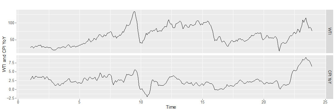
Figure 1: Graph of WTI and CPI YoY time series from 2000-2022.

3.2.Data Transformation

To fit the WTI and CPI YoY time series into an ARIMA model, the study first examines stationarity using the ADF test. Table 2 lists the ADF test results for the two time series before and after the first difference. Since the p-value for both time series is less than the critical value after taking the first difference, WTI and CPI YoY first difference time series are stationary.

Table 2: ADF test for WTI and CPI YoY before and after first difference.

3.3.Fitting into the ARIMA model

After finding stationary time series for WTI and CPI YoY, it is safe to identify ARIMA models and estimate the parameters for two series.

3.3.1.Single variable series ARIMA model

Table 3 shows the results obtained from automatically fitted ARIMA models for two series using R. Table 4 shows the outcomes from the Ljung-box test of residuals.

Table 3: Results from ARIMA models for WTI and CPI YoY time series.

Table 4: Residual test for ARIMA (1,1,0) and ARIMA (2,1,2)(1,0,0) [12] with drift.

The p-value for ARIMA (1,1,0) is greater than 0.05, and the residuals exhibit minimal autocorrelation, indicating a resemblance to white noise. This implies that the model fits well with the WTI time series. Based on the estimation of ARIMA (1,1,0) parameters, the model can be expressed as follows:

\( ∆{WTI_{t}}=0.3494∆{WTI_{t-1}}+{ε_{t}}\ \ \ (6) \)

However, for ARIMA (2,1,2)(1,0,0) [12] with drift, the p-value falls below the critical value, indicating that the residuals exhibit significant autocorrelation. The model is inappropriate for the CPI YoY time series.

3.3.2.Two variable series ARIMA model

By considering the correlation between WTI crude oil price and inflation, CPI YoY can be better forecasted by combining two time series to better capture the lags. Table 5 shows the results of ARIMA and dynamic regression models automatically fitted by R using two series. While the ARIMA model uses the original data from the two series, the dynamic regression model uses the fitted values from ARIMA (1,1,0) for the WTI series as the independent variable.

Table 5: Results from ARIMA models for CPI YoY by combining with WTI series.

Table 6: Residual test for ARIMA (0,1,2)(1,0,2) [12] errors and ARIMA (3,1,2)(2,0,0) [12] errors.

The information criteria shows ARIMA (0,1,2)(1,0,2) [12] errors is a better fit compared to ARIMA (3,1,2)(2,0,0) [12] errors. From Table 5, the automatically fitted ARIMA model has bigger log-likelihood, and smaller AIC, AICc, and BIC. Moreover, from Table 6, the residual result shows that the p-value is bigger, suggesting that the residual distribution is not significantly different from white noise. The estimated parameters for ARIMA (0,1,2)(1,0,2) [12] errors are listed in Table 7. The graph of fitted values for the CPI YoY forecast ideal model and real values are shown in Figure 2.

Table 7: Estimated parameters for ARIMA (0,1,2)(1,0,2) [12] errors.

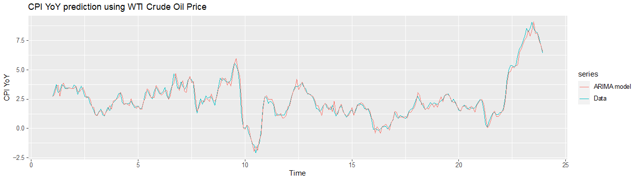
Figure 2: Real CPI YoY values and fitted values from ARIMA (0,1,2)(1,0,2)[12] errors.

3.4.Forecast

Finally, the optimal model for CPI YoY can predict future values using the known monthly average WTI crude oil price, updated until June 2023. Table 8 shows the monthly forecast for CPI YoY along with the real CPI YoY values recorded from January 2023 to June 2023. Figure 3 shows the CPI YoY prediction plot, which indicates a decreasing trend in 2023.

Table 8: Future forecast of CPI YoY from ARIMA (0,1,2)(1,0,2) [12] errors model.

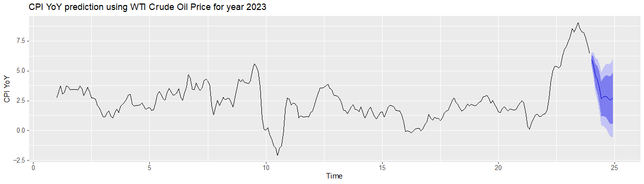
Figure 3: Forecast CPI YoY values from ARIMA (0,1,2)(1,0,2) [12] errors.

4.Discussion

Based on the results, the ARIMA (0,1,2)(1,0,2) [12] errors model is powerful in capturing the inner relationship between WTI crude oil price and CPI YoY. The oil price coefficient is positive and has small standard errors, indicating a positive relationship between the two variables. The positive coefficient implies a direct impact or correlation between the exogenous variable and the dependent variable.

The study also finds out that the automatic ARIMA model performs better compared to the dynamic regression model in fitting CPI YoY values. The comparative advantage can be credited to the model’s simplicity and ability to capture time series patterns. By employing algorithmic techniques to determine the most suitable values for the ARIMA parameters (p, d, q), the model automatically detects and incorporates seasonality in the data. This is particularly useful when analyzing time series data with periodic patterns. Moreover, it demonstrates the flexibility in exogenous variables. The automatic ARIMA model enables the incorporation of additional factors that improve forecasting accuracy and capture additional explanatory power.

5.Conclusion

This study uses monthly data that encompasses a period starting from January 2000 to December 2022. The result verifies the predictive power of WTI crude oil price on U.S. inflation. The ARIMA model and regression with the ARIMA errors model are engaged to forecast CPI YoY. The ideal model is selected based on how well it explains the stochastic variance in the data. By using the inner correlation between WTI crude oil price and inflation, ARIMA (0,1,2)(1,0,2) [12] errors is selected as an ideal model. Compared to the automatically generated ARIMA model that predicts based on time series patterns in CPI YoY historical data, the ideal model that combines WTI crude oil price performs better in accuracy.

Using ARIMA (0,1,2)(1,0,2) [12] errors, the study gives the inflation forecast result for 2023. The model prediction for CPI YoY value from January 2023 to June 2023 demonstrates a remarkable predictive effect. The real values fall into prediction intervals and the CPI YoY point forecast values show the same deflationary tendency. It provides a reference and basis to satisfy the needs of government, investors, and consumers to formulate policies and make financial decisions, which helps the macroeconomic operation and contributes to a good economic order.

However, the proposed model only considers WTI crude oil price as a single endogenous variable. While using WTI crude oil price as a predictor demonstrates a certain level of predictive power, exploring alternative models such as vector autoregression (VAR) or machine learning algorithms may provide more accurate and robust inflation forecasts. Future research can improve the model and forecast accuracy by incorporating other relevant factors, such as interest rates, employment data, and global economic indicators.

References

[1]. Nademi, A., & Nademi, Y. (2018). Forecasting crude oil prices by a semiparametric Markov switching model: OPEC, WTI, and Brent cases. Energy Economics, 74, 757–766. https://doi.org/10.1016/j.eneco.2018.06.020
[2]. Alturki, S., & Olson, E. (2022). Oil sentiment and the U.S. inflation premium. Energy Economics, 114, 106317. https://doi.org/10.1016/j.eneco.2022.106317
[3]. Mensi, W., Rehman, M. U., Hammoudeh, S., Vo, X. V., & Kim, W. J. (2023). How macroeconomic factors drive the linkages between inflation and oil markets in global economies? A multiscale analysis. International Economics, 173, 212–232. https://doi.org/10.1016/j.inteco.2022.12.003
[4]. Jean-Louis, C. O. M. B. E. S., & Lesuisse, P. (2022). Inflation and unemployment, new insights during the EMU accession. International Economics. https://doi.org/10.1016/j.inteco.2022.09.004
[5]. Caldara, D., Conlisk, S., Iacoviello, M., & Penn, M. (2022). The Effect of the War in Ukraine on Global Activity and Inflation. FEDS Notes, 2022(3141). https://doi.org/10.17016/2380-7172.3141
[6]. Zakaria, M., Khiam, S., & Mahmood, H. (2021). Influence of oil prices on inflation in South Asia: Some new evidence. Resources Policy, 71, 102014. https://doi.org/10.1016/j.resourpol.2021.102014
[7]. Wang, Y. S., & Chueh, Y. L. (2013). Dynamic transmission effects between the interest rate, the US dollar, and gold and crude oil prices. Economic Modelling, 30, 792–798. https://doi.org/10.1016/j.econmod.2012.09.052
[8]. Salisu, A. A., & Isah, K. O. (2018). Predicting US inflation: Evidence from a new approach. Economic Modelling, 71, 134–158. https://doi.org/10.1016/j.econmod.2017.12.008
[9]. Chou, K. W., & Tseng, Y. H. (2011). Pass-through of oil prices to CPI inflation in Taiwan. International Research Journal of Finance and Economics, 69(69), 73-83.
[10]. Katircioglu, S. T., Sertoglu, K., Candemir, M., & Mercan, M. (2015). Oil price movements and macroeconomic performance: Evidence from twenty-six OECD countries. Renewable and Sustainable Energy Reviews, 44, 257–270. https://doi.org/10.1016/j.rser.2014.12.016
[11]. Lu, Y., & AbouRizk, S. M. (2009). Automated Box–Jenkins forecasting modelling. Automation in Construction, 18(5), 547–558. https://doi.org/10.1016/j.autcon.2008.11.007
[12]. Rob J Hyndman and George Athanasopoulos. (2021). Chapter 10 Dynamic regression models | Forecasting: Principles and Practice (3rd ed). In otexts.com. Otexts. https://otexts.com/fpp3/dynamic.html
Cite this article
Liu,Y. (2023). Time Series Modeling and Forecasting of US Consumer Price Index Using WTI Crude Oil Price. Advances in Economics, Management and Political Sciences,48,125-133.
Data availability
The datasets used and/or analyzed during the current study will be available from the authors upon reasonable request.
Disclaimer/Publisher's Note
The statements, opinions and data contained in all publications are solely those of the individual author(s) and contributor(s) and not of EWA Publishing and/or the editor(s). EWA Publishing and/or the editor(s) disclaim responsibility for any injury to people or property resulting from any ideas, methods, instructions or products referred to in the content.
About volume
Volume title: Proceedings of the 2nd International Conference on Financial Technology and Business Analysis
© 2024 by the author(s). Licensee EWA Publishing, Oxford, UK. This article is an open access article distributed under the terms and
conditions of the Creative Commons Attribution (CC BY) license. Authors who
publish this series agree to the following terms:
1. Authors retain copyright and grant the series right of first publication with the work simultaneously licensed under a Creative Commons
Attribution License that allows others to share the work with an acknowledgment of the work's authorship and initial publication in this
series.
2. Authors are able to enter into separate, additional contractual arrangements for the non-exclusive distribution of the series's published
version of the work (e.g., post it to an institutional repository or publish it in a book), with an acknowledgment of its initial
publication in this series.
3. Authors are permitted and encouraged to post their work online (e.g., in institutional repositories or on their website) prior to and
during the submission process, as it can lead to productive exchanges, as well as earlier and greater citation of published work (See
Open access policy for details).