1. Introduction

1.1. Research Background and Significance

One of the most challenging problems that 21st-century society faced is climate change. The temperature has been increasing unnaturally during the past 50 years. The decade from 2010 to 2020 has been recorded as the warmest in history [1].

The impacts of these temperature changes extend beyond the environment and have far-reaching consequences for various industries. Higher temperatures bring various effects. For instance, heat waves tend to occur more frequently and last longer, causing diseases such as heat stroke or even death [1]. Furthermore, the accumulation of air pollutants from industrialization has disrupted the crucial interaction between photosynthesis and ultraviolet rays, contributing to the exacerbation of global warming [2]. Data from the National Aeronautics and Space Administration (NASA) indicates that carbon dioxide levels in the atmosphere have surpassed 420 parts per million (ppm) [3]. Consequently, its influence on the financial market has been growing as well. According to research on climate finance, climate change has become one of the most significant risk sources to the financial system. For example, it damages the infrastructure due to high temperatures [4].

Nevertheless, along with challenges, rising temperatures also present new opportunities within the stock market. As more regulatory burdens have been published by anticipated legislation to mitigate the negative impact that climate change brought, more financial expenditures corporations must pay. According to the Congressional Budget Office statistics, one recently proposed climate bill has cost firms approximately 100 billion dollars in one year [5]. Besides, the transition to a greener economy has created a new landscape for investment, generating potential profit sources.

Given this context, the relationship between rising temperatures and the stock market has attracted considerable attention in recent years. Furthermore, if the current pace of temperature rise continues. By 2100, the average global temperature is predicted to rise by 4 to 12 degrees Fahrenheit [1]. This underscores the urgency of understanding and analyzing the intricate relationship between temperature changes and the stock market.

1.2. Literature Review

Earlier research primarily exploring the correlation between the stock market and climate change relied on event study methodologies, such as the Hamilton events in 1995 and the Fisher-Vanden and Thorburn accident in 2011 [6]. These studies mainly examine the immediate impact of negative environmental performance on associated companies and their stocks in the short term.

Another research direction examines climate change's impacts by using index and portfolio levels [6]. For instance, research conducted by a team led by Papadamou examines the reactions of a sustainability stock index as the STOXX Global ESG Environmental Leaders Index, to major natural disasters caused by climate change, such as wildfires [7]. The study found that new information on environmental issues could also draw the public's attention. Moreover, investor preferences may depend not only on climate change but also on investor sentiment. Investors prefer sustainable stocks and sell them out when environmental awareness diminishes. Neo-sustainable investors also play a significant role in accelerating the buying process. For instance, they would increase their environmental awareness and turn into sustainable investors when traditional investments are perceived as riskier [7].

These studies proposed that with the assistance of climate-related policy and events, it could intensify the public's attention, which would encourage investors to allocate money to companies listed on sustainability stock indices. In this case, investors can counterbalance the negative effects and generate profits.

1.3. Content and Framework

The article aims to analyze the influence of rising temperatures on the stock market by examining the temperature change and performance of the S&P 500. The performance reflects the nature that the changing temperature brought to the stock market to some extent. The research is based on real-world data, focusing on the methodology employed and the results obtained. Additionally, the article provides further discussion on the relationships identified. By exploring the complex interplay between climate change and financial markets, this research seeks to contribute to understanding how temperature fluctuations can influence market dynamics and provides suggestions.

2. Methodology

The data used in the study was collected over 50 years, from 1972 to 2022, representing the monthly temperature of North America based on the mean values from all 48 states. The monthly temperature was collected using the land temperature, ignoring the fluctuations in ocean temperature. To make the data more accurate, the study primarily focused on data from the United States, sourced from reputable climate databases, such as those provided by the National Centers for Environmental Information under the National Oceanic and Atmospheric Administration (NCEI-NOAA) [8]. The extensive time range assists in finding long-term trends and patterns in temperature fluctuations. The selected time range reflects the most significant fluctuation in temperature. Global annual temperatures have increased by approximately 1 to 2 degrees Fahrenheit during the 19th century, with a more pronounced escalation observed in the late 20th century [9].

The stock market that this study mainly focuses on is S&P 500 from 2013 to 2022, and the data collected are from Federal Reserve Economic Data (FRED) to ensure authenticity [10]. Worth noticing is that for both variables, the data ignore the year 2023 because including incomplete data may lead to outliers and biases.

The descriptive statistics for the temperature time series covering 1972 to 2022 are shown in Table 1. The dataset contains 600 observations, with the highest monthly temperature recorded as 76.24 degrees Fahrenheit in 2022 and the lowest monthly temperature recorded as 25.50 degrees Fahrenheit in 1975.

Table 1: Descriptive statistics of Monthly temperature (1972-2022).

The research is divided into two main sections. The first part primarily focuses on the monthly temperature from 1972 to 2022 and finding its best-fitted ARIMA model. Based on the monthly temperature and S&P 500 statistics from 2013 to 2022, the second part focuses on investigating the regression models for these two variables. Moreover, using different regression models to make predictions and compare these models based on fitted values predicted by the ARIMA model. It is predicted that the temperature will impact the stock markets as S&P 500.

3. Results

The time series plot of monthly temperature in North America from 1972 to 2022 is shown in Figure 1. The plot shows strong seasonality from the characteristic of its natural data, and it is difficult to analyze its overall trend.

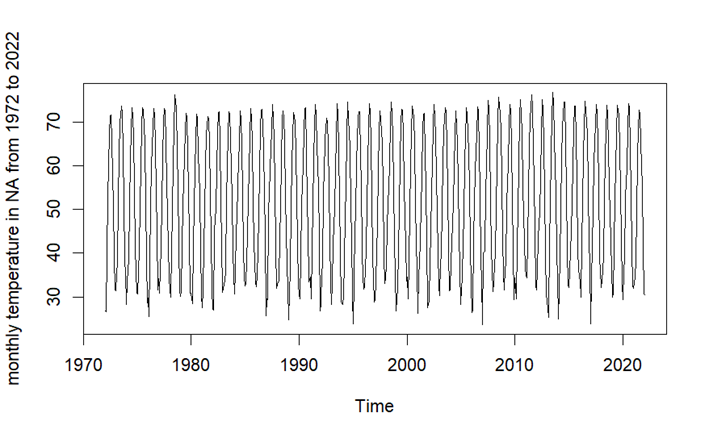
Figure 1: Monthly temperature in North America from 1972 to 2022.

Figure 2 illustrates the plot of seasonal differenced time series. The mean and variance of the differenced data are constant, indicating a lack of time-dependent structure and decreasing seasonality.

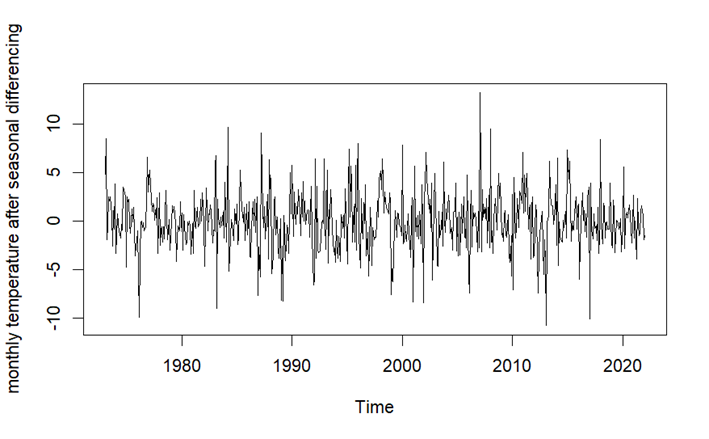
Figure 2: Monthly temperature in North America from 1972 to 2022 after seasonal differencing.

As indicated in Table 2, the study uses the Augmented Dickey-Fuller (ADF) Test to check its stationarity. The resulting p-value is 0.01, below the significance level of 0.05. The investigation thus suggests the monthly temperature time series is stationary and rejects the null hypothesis.

Table 2: ADF Test of monthly temperature (1972-2022).

After applying seasonal differencing, Figures 3 and 4 show the Autocorrelation Function (ACF) and Partial Autocorrelation Function (PACF). Most spikes in both figures fall within the confidence interval, indicating no significant autocorrelation issue. The results of the plots support the stationarity of the adjusted time series and suggest its suitability for fitting an ARIMA model.

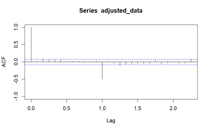
Figure 3: ACF plot after seasonal differencing.

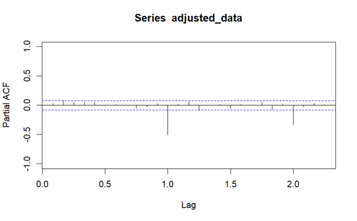
Figure 4: PACF plot after seasonal differencing.

With the lowest AIC, AICc, and BIC values, Table 4 shows the best fitting ARIMA model outcome. Among the models that have been examined, the ARIMA (2,0,2) (2,1,0) [12] with the drift model effectively reflects the underlying dynamics and patterns of the monthly temperature data.

Table 3: Estimation of ARIMA (2,0,2) (2,1,0) [12] with drift parameters.

The Ljung-Box test result indicates that the p-value is lower than 0.05. Since the fluctuation in the residuals plot is large, the residuals have significant autocorrelation.

Table 4: Results from Ljung-Box test of residuals from ARIMA (2,0,2) (2,1,0) [12].

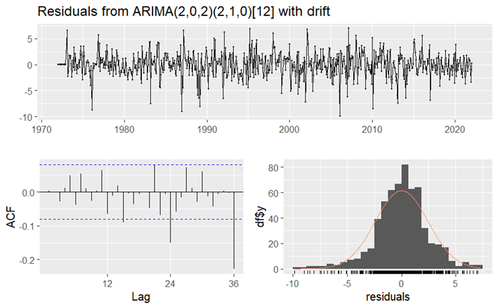
Figure 5: Residual result from ARIMA (2,0,2) (2,1,0) [12].

Figure 6 displays the forecast with the ideal model as ARIMA (2,0,2) (2,1,0) [12]. Using the seasonal naive forecast method efficiently utilizes historical seasonal patterns to make accurate predictions, making it a valuable tool for seasonal data analysis. The use of the ARIMA (2,0,2) (2,1,0) [12] model with the seasonal naive forecast method provides valuable insights into the future trends of the monthly temperature, assisting in decision-making and planning.

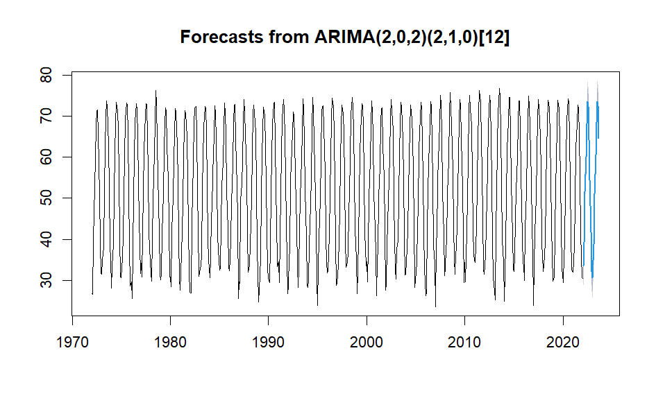
Figure 6: Forecast using seasonal naïve method of ARIMA (2,0,2) (2,1,0) [12].

Table 5 shows the descriptive statistics of monthly temperature and S&P500 from August 2013 to May 2022. The relatively short time allows for a more focused analysis, as it is expected to exhibit a more stable and predictable relationship between the two variables regarding trends and correlations.

Table 5: Descriptive statistics of monthly temperature and S&P 500 (2013-2022).

In the second phase of the data analysis, the objective is to determine a suitable model for the monthly temperature time series observed from 2013 to 2022 and use the fitted value to regress S&P 500 and monthly temperature. By doing so, it analyzes the correlation between these two. Figure 7 presents a time series plot of monthly temperature and S&P 500 from 2013 to 2022. The plot of monthly temperature remains high seasonality, while the S&P 500 has an overall increasing trend.

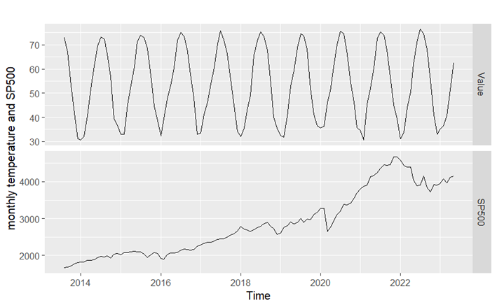
Figure 7: Time series plot of monthly temperature and S&P 500 (January 2014 – December 2022).

Next, this study tests the stationarity of monthly temperature time series using ADF Test to generate a fit model for monthly temperature from 2013 to 2022. Table 6 shows the result for determining the stationarity, which indicates the p-value of 0.01. As a result, the null hypothesis been rejected. It is a stationary time series.

Table 6: ADF Test for monthly temperature (2013-2022).

Using the “autoarima” code in R, the study finds that the best-fitted model for the combination of monthly temperature and S&P 500 is ARIMA (0,0,5) (1,0,1) [12] errors. Table 7 indicates that the p-value obtained from the Ljung-Box test is significantly lower than 0.05. This finding provides evidence of autocorrelation issues within the time series.

Table 7: Results from Ljung-Box test of residuals from ARIMA (0,0,5) (1,0,1) [12].

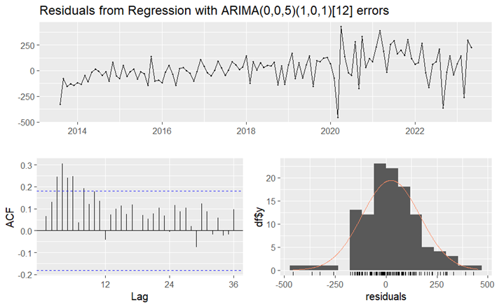
Figure 8: Residuals results from ARIMA (0,0,5) (1,0,1) [12] error.

Then, using the statistic of monthly temperature from 2013 to 2022, the study finds its best fitted model as ARIMA (0,0,0) (2,1,0) [12]. By conducting the residual plot and Ljung-Box test, as shown in Table 8 and Figure 9, the results also show autocorrelation.

Table 8: Results from Ljung-Box test of residuals from ARIMA (0,0,0) (2,1,0) [12].

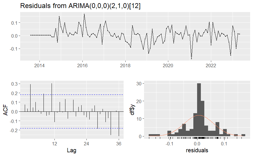
Figure 9: Residuals results from ARIMA (0,0,0) (2,1,0) [12].

The study used two models to fit the linear and dynamic regression models. The linear regression model using the ARIMA (0,0,0) (2,1,0) ^[12] model. The dynamic regression model using the ARIMA (0,1,0) errors as the best-fitted model using statistics of S&P 500 as shown in Table 9 and Figure 10 and presents that the model has little autocorrelation.

Table 8. Results from Ljung-Box test of residuals from ARIMA (0,1,0) errors.

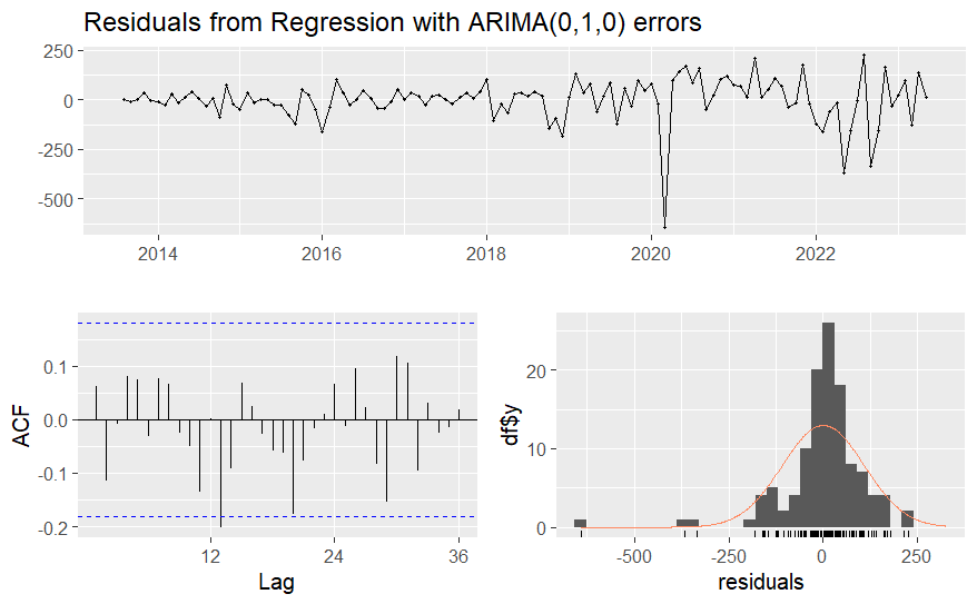
Figure 10: Residuals results from ARIMA (0,1,0) errors.

Since the fitted model using the Linear regression model shows more autocorrelation, using the Dynamic regression model provides less autocorrelation. Moreover, it provides a more precise understanding of the relationship between the variables over time, making it a more improved forecasting model.

Figure 11 illustrates a comparison between the forecasts generated by the dynamic regression model ARIMA (0,1,0) errors, the linear regression model as ARIMA (0,0,0) (2,1,0) [12] errors, and the actual real-life statistics.

The forecast result using ARIMA (0,1,0) errors is shown in Figure 12. The dynamics regression model generally shows the best result for describing and forecasting the impact of temperature changes in the S&P 500.

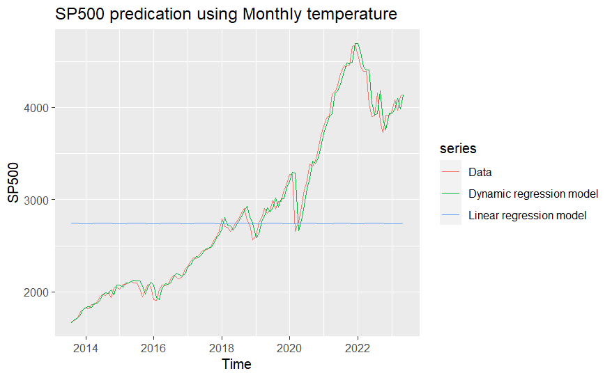
Figure 11: Forecast result from different model.

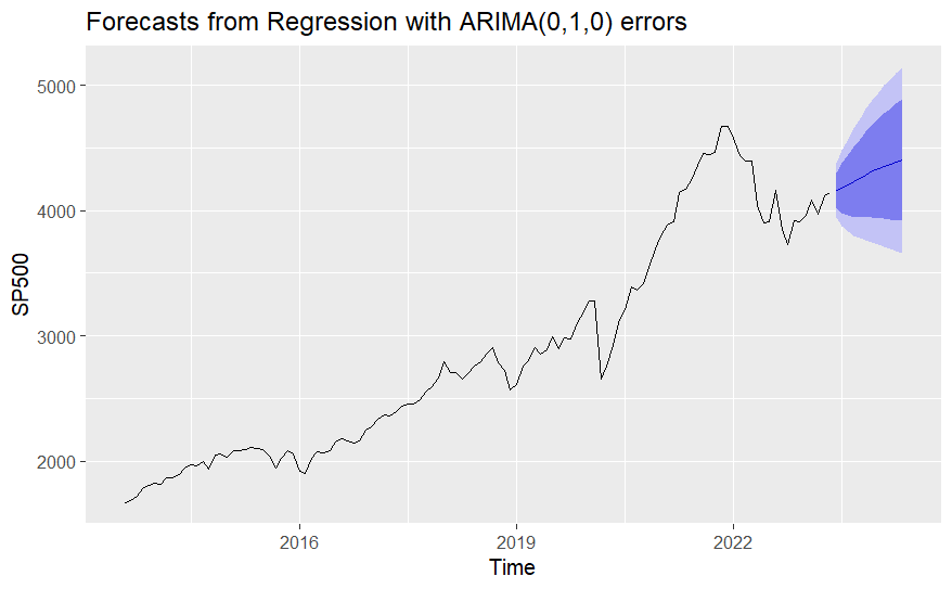
Figure 12. Forecast result using ARIMA (0,1,0) errors.

4. Discussion

The results show that the temperature has no significant effects on S&P 500 based on the forecasting result from the Linear regression model. In contrast, the temperature positively affects S&P 500 based on the Dynamic regression model. The findings support the hypothesis that temperature fluctuations influence the stock market and are associated with a positive impact on its performance.

There are several possible reasons for the finding that rising temperature positively influences performance. First, a more positive sentiment of investors tends to be triggered by higher temperatures. In this case, the sentiments could transform into higher stock demand and increase the share prices. Moreover, the changing temperature provides opportunities for certain new industries. For example, corporations in the renewable energy sector or companies that provide certain solutions to alleviate the negative influences of climate change benefit from the shift. The booming of the shares from specific areas contributes to a positive performance of the S&P 500. Furthermore, as the precipitation of these corporations increases, investors tend to invest more in them and increase their share prices. Additionally, temperature increases often prompt governments to introduce measures and policies to mitigate climate change. These regulations can create new market opportunities and incentivize investments in environmentally friendly technologies and practices. Companies that align with these regulations may experience positive effects.

The results of this study align with Bolton's research, which investigated the connection between carbon emissions and cross-sectional stock returns in the United States. The study revealed that firms with higher carbon emissions generally experienced larger stock returns while holding other factors, such as the constant book-to-market and other return predictors [11]. This relationship can be attributed to the positive impact of carbon dioxide on greenhouse effects, which in turn contributes to rising temperatures. Therefore, the positive influence observed in this article aligns with these previous findings.

Though the study has considered the relationship from different angles using different models, some limitations remain. The first limitation is with the original data choice in model fitting. The used data only consider the data of North America to make it more related to the S&P 500. To improve that, a larger sample should be included to increase the precision of the analysis. Additionally, the temperature observation data only includes the land temperature statistic instead of the combination of land and ocean temperature. More research should be done to ensure the feasibility of a combination statistic and the way to imply it. Moreover, the monthly temperature selected is from 1972, while drastic temperature change started in the mid-18th century with the beginning of the industrial revolution. The improvement could be selecting a longer time range for the analysis while maintaining the precision and consistency of statistics. It is advantageous to consider other factors that influence this relationship to improve the analysis. Besides, conducting a more detailed analysis of the specific periods or seasons when temperature fluctuations have the strongest influence on the S & P 500 could increase the applicability of the study result.

5. Conclusion

In conclusion, this study aimed to explore the correlation between rising temperatures and the S&P 500 index. The analysis is based on historical data on temperature change in North America and the index. Several findings have been made by applying various econometric models, including ARIMA and regression models. The study revealed a significant positive relationship between temperature changes and stock market performance using the dynamic regression model used in forecasting, indicating that rising temperatures positively influence the S&P 500 index.

This finding suggests that rising temperature is an important factor that should be considered in investment decision-making processes. The implications of this study extend beyond the realm of finance. The findings are relevant for policymakers seeking to address climate-related risks and develop effective mitigation strategies. Additionally, investors can benefit from deeper comprehension of the interplay between rising temperatures and stock market performance, enabling them to make informed investment decisions in a changing climate.

However, there are still limitations to this study. The analysis focused on the S&P 500 index and may need to capture the nuances and dynamics of other stock markets fully. Moreover, the research relied on historical data. Though the forecasting has been done, some potential future changes in climate patterns and regulations may need to be addressed. Additionally, the statistic used has unavoidable autocorrelation issues, especially in the statistics of monthly temperature. The issue cannot be eliminated using the transformation method of logarithm and differencing in the data. These problems may be caused by containing outliers and not applying the appropriate model. For further study, there may be some suggestions to address these challenges. Different models and a wider range of statistics could be applied in the future to mitigate these problems. It would be beneficial to explore the influence of climate change on specific industry sectors and analyze the differential effects across different stock indices. Additionally, incorporating forward-looking climate scenarios and conducting scenario analysis can provide more comprehensive insights into the potential risks and opportunities linked with climate change. As risks continue to escalate, further research in this field is crucial for effective risk management and sustainable investment practices.

References

[1]. US. (2020b). Higher Temperatures | A Student’s Guide to Global Climate Change | US EPA. Epa.gov. https://archive.epa.gov/climatechange/kids/impacts/signs/temperature.html. last accessed 2023/7/01.
[2]. Kelp, Makoto M., Andrew P . Grieshop, Conor CO Reynolds, Jill Baumgartner, Grishma Jain, Karthik Sethuraman, and Julian D. Marshall. (2018). Real-time indoor measurement of health and climate-relevant air pollution concentrations during a carbon-finance-approved cookstove intervention in rural India. Development Engineering 3: 125–32.
[3]. Fang, Zheng, Jianying Xie, Ruiming Peng, and Sheng Wang. (2021). Climate Finance: Mapping Air Pollution and Finance Market in Time Series. Econometrics 9: 43. https://doi.org/10.3390/econometrics9040043. last accessed 2023/7/05.
[4]. Bee-Hoong Tay. (2023). Climate change and stock market: a review. IOP Conf. Ser.: Earth Environ. Sci. 1151 012021. last accessed 2023/7/07.
[5]. Timothy Beatty and Jay P. Shimshack (2010) “The Impact of Climate Change Information: New Evidence from the Stock Market,” The B.E. Journal of Economic Analysis & Policy: l. 10, 105.
[6]. El Ouadghiri, Imane, et al. (2021) “Public Attention to Environmental Issues and Stock Market Returns.” Ecological Economics, 180, 106836,
[7]. Kollias, C., Papadamou, S., 2016. Environmentally responsible and conventional market indices’ reaction to natural and anthropogenic adversity: a comparative analysis. J. Bus. Ethics 138 (3), 493–505.
[8]. “Global Time Series | Climate at a Glance | National Centers for Environmental Information (NCEI).” www.ncei.noaa.gov/access/monitoring/climate-at-a-glance/global/time series/northAmerica/land/all/1/1850-2023. last accessed 2023/7/01.
[9]. MacMillan, Amanda, and Jeff Turrentine. “Global Warming 101.” NRDC, 7 Apr. 2021, www.nrdc.org/stories/global-warming-101#warming. last accessed 2023/7/01.
[10]. “S&P 500.” Fred.stlouisfed.org, 20 Apr. 2020, fred.stlouisfed.org/series/SP500. https://fred.stlouisfed.org/series/SP500. last accessed 2023/7/01.
[11]. Bolton, P., & Kacperczyk, M. T. (2019). Do Investors Care about Carbon Risk? SSRN Electronic Journal, 142(2).
Cite this article
Xiao,J. (2023). Time Series Analysis of Climate Change & Its Relationship with Stock Price. Advances in Economics, Management and Political Sciences,49,45-57.
Data availability
The datasets used and/or analyzed during the current study will be available from the authors upon reasonable request.
Disclaimer/Publisher's Note
The statements, opinions and data contained in all publications are solely those of the individual author(s) and contributor(s) and not of EWA Publishing and/or the editor(s). EWA Publishing and/or the editor(s) disclaim responsibility for any injury to people or property resulting from any ideas, methods, instructions or products referred to in the content.
About volume
Volume title: Proceedings of the 2nd International Conference on Financial Technology and Business Analysis
© 2024 by the author(s). Licensee EWA Publishing, Oxford, UK. This article is an open access article distributed under the terms and
conditions of the Creative Commons Attribution (CC BY) license. Authors who
publish this series agree to the following terms:
1. Authors retain copyright and grant the series right of first publication with the work simultaneously licensed under a Creative Commons
Attribution License that allows others to share the work with an acknowledgment of the work's authorship and initial publication in this
series.
2. Authors are able to enter into separate, additional contractual arrangements for the non-exclusive distribution of the series's published
version of the work (e.g., post it to an institutional repository or publish it in a book), with an acknowledgment of its initial
publication in this series.
3. Authors are permitted and encouraged to post their work online (e.g., in institutional repositories or on their website) prior to and
during the submission process, as it can lead to productive exchanges, as well as earlier and greater citation of published work (See
Open access policy for details).