1. Introduction

Risk and expected return are the two core issues that investors are most concerned about. Therefore, judging the return and risk of an asset investment and achieving the optimal asset allocation on the basis of balancing the two indicators is what every investor wants. effort to achieve. In this context, Markowitz published a work called “Portfolio Selection” in 1952, and the Mean-Variance Model has been officially launched since then. In this article, Markowitz proposed to use the mean value of risky assets to represent the expected rate of return, and the variance (or standard deviation) to represent the risk level, and to explore asset portfolio and selection issues accordingly [1]. The key role of this theory is that it can guide investors to invest funds in various securities according to a certain proportion, and achieve the minimum risk when the given expected return is realized, or the maximum return when the given risk is given.

Since the mean-variance model was proposed, there has been a lot of research around it in the academic circles. For instance, based on an imperfect market, Xie et al. explored the continuous-time mean-variance portfolio selection model comprising multi-risk assets and a liability. They obtained the optimal dynamic strategy as well as the mean-variance efficient frontier from their findings [2]. Zhang Aiguo et al. studied the most profitable securities with the use of Markowitz's mean-variance model, and they created a mean-variance model for optimal asset allocation using the same methodology [3]. Some scholars broke the assumption that the relevant parameters were known in the previous research, and focused on the parameter uncertainty and the dynamic mean-variance model in Bayesian learning based on the martingale method, and finally obtained the optimal solution and efficient frontier [4]. Wang Xiaoqin et al. introduced a non-concave and non-convex transaction cost function in the article, and by embedding it into the model, they obtained the mean-variance-lower half-variance portfolio model, and obtained good results [5]. This paper draws on the existing research, uses the data of 10 stocks listed on the Shenzhen Stock Exchange from 2019 to 2020, uses the Markowitz mean-variance model, implements quadratic programming in EXCEL, and obtains the set expected rate of return. The corresponding weights and minimum standard deviations of each security are obtained, and the efficient frontier is obtained.

\( {σ_{p}}=\sum _{i=1}^{n}{w_{i}}{w_{j}}cov({r_{i}},{r_{j}}) \) (1)

\( E({r_{i}})=\frac{\sum _{i=1}^{m}{r_{i}}}{m} \) (2)

\( E({r_{i}}) \) is the mean of porffolio return rate series, \( {σ_{p}} \) is the standard deviation. \( {w_{i}} \) is the weight of stock, \( {r_{i}} \) is the seires of stock return rate.

2. Portfolio Allocation Implementation Process

Here, we will use 600519.SH Kweichow Moutai, 301073.SZ Junting Hotel, 600104.SH SAIC, 002475.SZ Luxshare Precision, 300750.SZ Ningde Ara and 601398.SS Industrial and Commercial Bank of China Limited as an example to construct a portfolio.

First, we obtain the daily closing price data of the above four stocks from 2012 to now, and draw the stock price data as a curve:

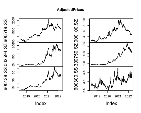
Fig. 1. Adjusted price of four stocks from 2018-01-01.

Further, the sequence of four stocks can be calculated:

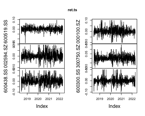
Fig. 2. Daily return rate of four stocks from 2018-01-01.

3. Model Assessment

On the basis of being able to define investment risks and returns, it is possible to return to the original intention of the mean-variance theory, which is to obtain a set of weights so that the risk-return ratio of the portfolio configured with the weights can reach the optimal state. Regardless of how to find this optimal set of weights, if we randomly generate a large number of weight combinations and configure the above four stocks according to these weight combinations, then we can get the risks and returns corresponding to each combination. If the risk is on the horizontal axis, and plotting these combination points on the vertical axis. Model explanation: In the case of uncertain weights, in countless investment portfolios, as long as a given risk level is given, we can always find a superior investment portfolio. The goal of the so-called "ideal investment portfolio" is to achieve a constant level of risk. It is possible to say that the portfolio that has the highest return is also the portfolio that has the lowest risk for a given level of return, and the curve that is produced by the points on the optimal portfolio that correspond to different risk levels is known as the Efficient Frontier.

## ## Title:## Portfolio Constraints## ## Lower/Upper Bounds:## 600519.SS 002594.SZ 600438.SS 000100.SZ 300750.SZ 600300.SS## Lower 0 0 0 0 0 0## Upper 1 1 1 1 1 1## ## Equal Matrix Constraints:## ceq 600519.SS 002594.SZ 600438.SS 000100.SZ 300750.SZ 600300.SS## Budget -1 -1 -1 -1 -1 -1 -1## attr(,"na.action")## Return ## 1 ## attr(,"class")## [1] "omit"## ## Cardinality Constraints:## 600519.SS 002594.SZ 600438.SS 000100.SZ 300750.SZ 600300.SS## Lower 0 0 0 0 0 0## Upper 1 1 1 1 1 1

## ## Title:## MV Portfolio Frontier ## Estimator: covEstimator ## Solver: solveRquadprog ## Optimize: minRisk ## Constraints: LongOnly ## Portfolio Points: 5 of 6 ## ## Portfolio Weights:## 600519.SS 002594.SZ 600438.SS 000100.SZ 300750.SZ 600300.SS## 1 0.0000 0.0000 0.0000 0.0000 0.0000 1.0000## 2 0.4489 0.0468 0.0249 0.1901 0.0148 0.2745## 3 0.3956 0.0748 0.0985 0.0890 0.1700 0.1721## 4 0.3372 0.1011 0.1715 0.0000 0.3264 0.0638## 6 0.0000 0.0000 0.0000 0.0000 1.0000 0.0000## ## Covariance Risk Budgets:## 600519.SS 002594.SZ 600438.SS 000100.SZ 300750.SZ 600300.SS## 1 0.0000 0.0000 0.0000 0.0000 0.0000 1.0000## 2 0.4437 0.0419 0.0217 0.1930 0.0119 0.2877## 3 0.3671 0.0832 0.1140 0.0779 0.2184 0.1395## 4 0.2310 0.1045 0.1917 0.0000 0.4433 0.0295## 6 0.0000 0.0000 0.0000 0.0000 1.0000 0.0000## ## Target Returns and Risks:## mean Cov CVaR VaR## 1 0.0005 0.0264 0.0593 0.0433## 2 0.0011 0.0172 0.0382 0.0260## 3 0.0016 0.0177 0.0383 0.0246## 4 0.0021 0.0204 0.0418 0.0279## 6 0.0031 0.0330 0.0649 0.0469## ## Description:## Thu Apr 21 20:03:38 2022 by user:

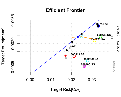
Fig. 3. Efficient forntier of the portfolio.

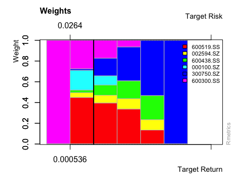
Fig. 4. The Weight of stocks without constraint

## ## Title:## Portfolio Constraints## ## Lower/Upper Bounds:## 600519.SS 002594.SZ 600438.SS 000100.SZ 300750.SZ 600300.SS## Lower 0.0 0.0 0.0 0.0 0.0 0.0## Upper 0.5 0.5 0.5 0.5 0.5 0.5## ## Equal Matrix Constraints:## ceq 600519.SS 002594.SZ 600438.SS 000100.SZ 300750.SZ 600300.SS## Budget -1 -1 -1 -1 -1 -1 -1## attr(,"na.action")## Return ## 1 ## attr(,"class")## [1] "omit"## ## Cardinality Constraints:## 600519.SS 002594.SZ 600438.SS 000100.SZ 300750.SZ 600300.SS## Lower 0 0 0 0 0 0## Upper 1 1 1 1 1 1

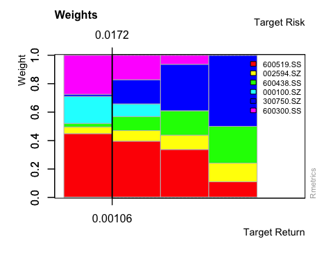
Fig. 5. The weight of stocks with constraint

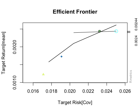
Fig. 6. Efficient Frontier of the portfolio

In addition to determining several important input variables, we also need to constrain the weight of each asset in the portfolio, including lower bound and upper bound constraints. This method is used to ensure portfolio diversity, reduce parameter estimation errors, and expand investment. It has been applied in terms of risk appetite and so on. Table 3 shows the minimum and maximum weights of each type of asset in the portfolio. We choose 0% as the minimum value of the allocation, because too low weights lose the meaning of reducing unsystematic risks; at the same time, we choose 50% as the the maximum value of the allocation, so that the allocation of each asset is more balanced and practical. Of course, for U.S. stocks, Hong Kong stocks and gold assets, for reasons such as risk reduction and foreign exchange quotas, their lower limit is at least 0%.

For a given six stocks, construct all possible combination configurations, and we can magically find that these combination points converge into a bullet-like graph. From the analysis in the figure, it can be concluded that the lower part of the bullet is invalid, because the combination below has a higher return than it under the same risk, so we do not take the combination below. With the same analytical framework, we can think that there is an optimal portfolio at the boundary above the bullet, which is also called the Markowitz efficient frontier. Of course, since the bullet boundary in the above figure is obtained by a finite number of simulations, the actual effective frontier is different from the boundary shown in the illustration.

Last but not least, we need to find a solution to the dilemma of how to obtain the ideal ratio of returns and risks while simultaneously diversifying hazards. In this case, there are two things to take into consideration: 1. Assume the least possible amount of investment risk in order to maximize the rate of return that is anticipated. 2. At an acceptable level of investment risk, to achieve maximum investment returns. Since the two ideas are essentially the same, here we only consider the first idea for modeling.

Since the two ideas are essentially the same, here we only consider the first idea for modeling

\( min μ=\sum _{i=1}^{n}{w_{i}}{w_{j}}cov({r_{i}},{r_{j}})s.t {r^{T}}w \)

\( =μ\sum _{i=1}^{n}{w_{i}}=1{w_{i}}≥0 \) (3)

According to the above model, we can solve a large number of portfolio points on the efficient frontier, and by fitting these points, the efficient frontier can be obtained.

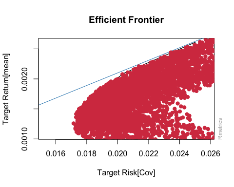
Fig. 7. The tangent return of the efficient frontier

## ## Title:## MV Portfolio Frontier ## Estimator: covEstimator ## Solver: solveRquadprog ## Optimize: minRisk ## Constraints: minW maxW ## Portfolio Points: 4 of 4 ## ## Portfolio Weights:## 600519.SS 002594.SZ 600438.SS 000100.SZ 300750.SZ 600300.SS## 1 0.4489 0.0468 0.0249 0.1901 0.0148 0.2745## 2 0.3956 0.0748 0.0985 0.0890 0.1700 0.1721## 3 0.3372 0.1011 0.1715 0.0000 0.3264 0.0638## 4 0.1106 0.1311 0.2583 0.0000 0.5000 0.0000## ## Covariance Risk Budgets:## 600519.SS 002594.SZ 600438.SS 000100.SZ 300750.SZ 600300.SS## 1 0.4437 0.0419 0.0217 0.1930 0.0119 0.2877## 2 0.3671 0.0832 0.1140 0.0779 0.2184 0.1395## 3 0.2310 0.1045 0.1917 0.0000 0.4433 0.0295## 4 0.0407 0.1105 0.2475 0.0000 0.6012 0.0000## ## Target Returns and Risks:## mean Cov CVaR VaR## 1 0.0011 0.0172 0.0382 0.0260## 2 0.0016 0.0177 0.0383 0.0246## 3 0.0021 0.0204 0.0418 0.0279## 4 0.0026 0.0250 0.0508 0.0352## ## Description:## Thu Apr 21 20:03:38 2022 by user:

4. Discussion

Markowitz’s mean-variance theory plays an important role in guiding investors’ investment. Once it was put forward, it attracted wide attention. Since then, there have been many studies on the mean-variance model, and scholars have made improvements on the basis of this model. A series of models are derived, such as mean-semivariance model, maximum and minimum model, etc. Although the mean-variance model has certain limitations, such as ideal assumptions and difficult operation, it is undeniable that it is still the most standard model in general securities portfolios, and it is also the most commonly used capital pricing theoretical model under uncertainty. Drawing on existing research, this paper first introduces the relevant content of the Markowitz mean-variance model, and takes this as a theoretical basis. The quadratic programming is realized in the middle, and the weight and minimum standard deviation of each asset under the set expected rate of return are obtained, and the effective frontier is obtained.

5. Conclusion

Markowitz's portfolio theory has long since been shown to be effective in practice, and as a result, it is widely utilized in portfolio selection and asset allocation. Developed securities markets are the primary focus of this theory. However, there has been a great deal of debate about whether or not the theory is appropriate for the stock market in our nation in the circles who are concerned with securities theory and practice in our country.

In its most basic form, an investment portfolio can be thought of as a collection of securities that have been assigned a particular investment ratio. Of course, it's possible to consider a single investment in the form of a portfolio, even if it only consists of one share.

When making an investment, individuals are, in essence, making a choice between the uncertain returns and the risks. Mean-variance analysis is employed by portfolio theory in order to characterize these two primary considerations. It is the weighted average of a single security's projected return and its investment ratio that is referred to as the "mean" of the portfolio's expected return. Dividends and appreciation in value are unavoidable components of stock returns. The term "variance" refers to the variation in the portfolio's return. The volatility of a portfolio's return standard deviation is what we refer to as its risk level.

References

[1]. Markowitz H M . Portfolio Selection[J]. The Journal of Finance, 1952, 7(1):77.
[2]. Xie S , Li Z , Wang S . Continuous-time portfolio selection with liability: Mean-variance model and stochastic LQ approach[J]. Insurance, 2008, 42(3):p.943-953.
[3]. C.S. Binkley, C.F. Raper and C.L. Washburn, Institutional ownership of US timberland: history, rationale, and implications for forest management, Journal of Forestry 94(9) (1996) 21–28.
[4]. R. Brazee and R. Mendelsohn, Timber harvesting with fluctuating prices, Forest Science 34 (1988) 359–372.
[5]. William N. Goetzmann. (2020) The Financial Analysts Journal and Investment Management. Financial Analysts Journal 76:3, pages 5-21.
Cite this article
Lin,Z. (2023). Mean-Variance Model Theory and Its Application in Chinese Stock Market. Advances in Economics, Management and Political Sciences,3,803-811.
Data availability
The datasets used and/or analyzed during the current study will be available from the authors upon reasonable request.
Disclaimer/Publisher's Note
The statements, opinions and data contained in all publications are solely those of the individual author(s) and contributor(s) and not of EWA Publishing and/or the editor(s). EWA Publishing and/or the editor(s) disclaim responsibility for any injury to people or property resulting from any ideas, methods, instructions or products referred to in the content.
About volume
Volume title: Proceedings of the 6th International Conference on Economic Management and Green Development (ICEMGD 2022), Part Ⅰ
© 2024 by the author(s). Licensee EWA Publishing, Oxford, UK. This article is an open access article distributed under the terms and
conditions of the Creative Commons Attribution (CC BY) license. Authors who
publish this series agree to the following terms:
1. Authors retain copyright and grant the series right of first publication with the work simultaneously licensed under a Creative Commons
Attribution License that allows others to share the work with an acknowledgment of the work's authorship and initial publication in this
series.
2. Authors are able to enter into separate, additional contractual arrangements for the non-exclusive distribution of the series's published
version of the work (e.g., post it to an institutional repository or publish it in a book), with an acknowledgment of its initial
publication in this series.
3. Authors are permitted and encouraged to post their work online (e.g., in institutional repositories or on their website) prior to and
during the submission process, as it can lead to productive exchanges, as well as earlier and greater citation of published work (See
Open access policy for details).