1. Introduction

The accuracy of prediction is one of the major characteristics of modeling. Without accurate output, the entire model would be pointless for those who take stock price forecasting as part of their investment consideration. Therefore, it is necessary to testify which model can predict the stock price with the highest accuracy.

Stock price prediction using machine learning has been a prevailing topic to research. Numbers of scientist did their research about stock price prediction by using machine learning and modeling [1, 2]. They analyzed the advantages of XGBoost model [3, 4], RNN model [5] and LSTM model [6-10], but they did not directly compare the accuracy between two models. This paper aims to compare two renowned models, XGBoost and LSTM, and to testify the accuracy they can perform under the different condition.

This paper sets up the dataset in three time periods and will apply those datasets to the XGBoost model and LSTM model. After predicting the stock prices in each model, a total of six figures would be generated and the RMSE value would be calculated. In the end, this paper will compare the changes in prediction along with the increase of the dataset’s size visually, and a table will be inserted to compare the RMSE values. In the end, this paper concluded that XGBoost model has higher accuracy in large-size dataset, and LSTM model has higher accuracy in small-size dataset.

2. Data and Methods

2.1. Data

To analyze the research, this paper is using the stock price of Chevron Corporation (also called CVX) found in Yahoo Finance. Three different time stamps were used and each of them is three years apart. The reason this paper sets them 3 years apart is that 3 years is the time that neither makes them irrelevant nor grows long enough to clearly see the impact of the data size on the models. Thus, starting from the date July 25th, 2023, the data size would be the stock price 3 years, 6 years, and 9 years apart from that date. Then, this paper collected seven variables about stock price from Yahoo Finance, they are: “Date”, “Open”, “High”, “Low”, “Close”, “Adj Close”, and “Volume”. In particular, the “Close”, which is the closing price of each trading day, is widely considered to best represent the fluctuation of the stock price among those variables. Thus, in all the following data and methods, this paper used the closing price in our estimation.

There are 2264 observations collected in 2014, 1509 observations collected in 2017, and 753 observations collected in 2020. The dataset since 2014 has the most observations. Therefore, in the following part of the article, this dataset will be called a “large-size dataset”. Similarly, the dataset since 2017 is called a “medium-size dataset”, and the dataset since 2020 is called a “small-size dataset”.

2.2. Method

In this paper, this paper used two models to predict the stock price of CVX. They are XGBoost and LSTM models. For each chosen year, this paper will apply those models to the same data set, calculating the RMSE and MSE values for comparison. Also, this paper will plot the result comparing the predicted value and actual value visually.

2.2.1. XGBoost

XGBoost stands for Extreme Gradient Boosting. It would combine the prediction of multiple individual models to create an accurate and robust prediction. Those individual models usually refer to the decision trees. The way that XGBoost functions is to create a single decision tree, and then create another decision tree trying to revise the mistakes that the previous decision tree made. This process shall be repeated many times and each new decision tree will try to correct the previous one. Then, the final predicted result is calculated by summing all the predictions of all the individual trees. The way it functions made XGBoost can manage the missing values. It can work with real-world data that contains gaps and does not need extensive preprocessing. Also, XGBoost works excellently in preventing overfitting by its Cross-validation function.

XGBoost model is based on the use of a Regression Tree (also called CART). The decision rule of CART is the same as the decision trees, but each leaf of CART has a weight. The weights are the predicted values for each leaf (See Figure 1).

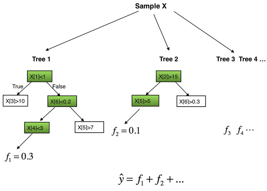
Figure 1: The explanation of the Tree Ensemble Model.

The result of the prediction would be the sum weight of each decision tree [11]. There are two decision trees in Figure 1. The output values at the bottom of the tree are the weights or the scores of the predicted value of each leaf. As inputting a set of data for prediction, those data would be partitioned based on the decision criteria of each internal node. The weight of each leaf would become the predicted output for those data.

In the equation above, \( {f_{k}} \) represents the regression trees, and “K” is the number of regression trees. The input data is \( {X_{i}} \) . The prediction output \( {ŷ_{i}} \) is the sum of the predicted values from K number of \( {f_{k}} \) regression trees.

2.2.2. LSTM

LSTM stands for Long Short-Term Memory. It is a type of recurrent neural network that can capture order dependencies in sequence prediction tasks [3]. Its capability to inherent capacity to retain and utilize past information makes LSTM particularly valuable in predicting stock prices [3]. The reason is that forecasting future stock prices heavily relies on analyzing the patterns in previous price movements (See Figure 2).

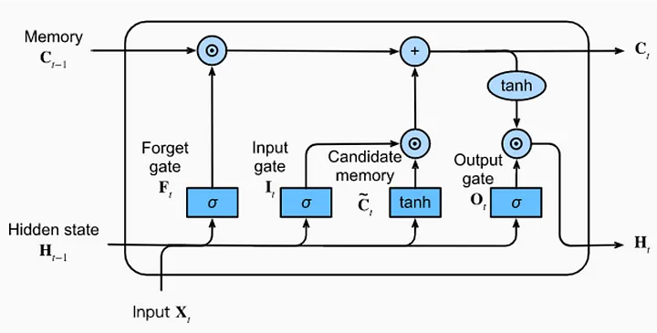
Figure 2: Architecture of an LSTM Unit

The LSTM architecture is made by a single LSTM unit that is composed of four feedforward neural networks. Each neural network includes one input layer and one output layer. Those input neurons would be connected to all the output neurons. Based on that, the LSTM unit incorporates four fully connected layers.

Among these four feedforward neural networks, three of them play a significant role in information selection. These three networks are the forget gate, the input gate, and the output gate. They are responsible for executing three essential memory management tasks: removing information from memory (forget gate), incorporating new information into memory (input gate), and utilizing the information already stored in memory (output gate). The last neural network is the candidate memory network. Its function is to generate fresh candidate information for potential insertion into the memory.

3. Result

3.1. XGBoost

For the XGBoost model, this paper extracted the “Close” price from the data frame and implemented a custom train-test split function. Then, the entire dataset is divided into training and testing subsets. Among them, 80 percent of the dataset is in training subsets, and the other 20 percent is in testing subsets. After the data preprocessing part, the objective is set as “reg:squarederror” for regression tasks and specified the number of estimators as 1000. Then, the training dataset is trained by the XGBoost model. This paper then sets the features to be x and the target to be y. After that, the model fits into the training data and makes the prediction based on it.

As a result, this paper plotted out the actual value and the predicted value below and calculated the RMSE and MSE value for years large, medium, and small-size dataset in the following Figures 3-5:

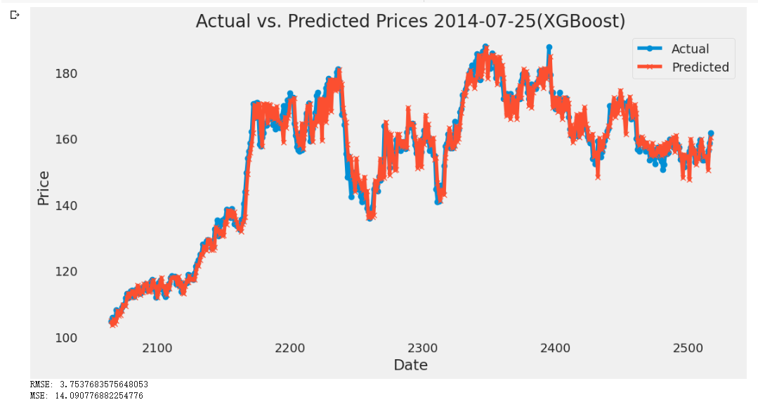
Figure 3: Plot of XGBoost Model of CVX from 2014-07-25 to 2023-07-25

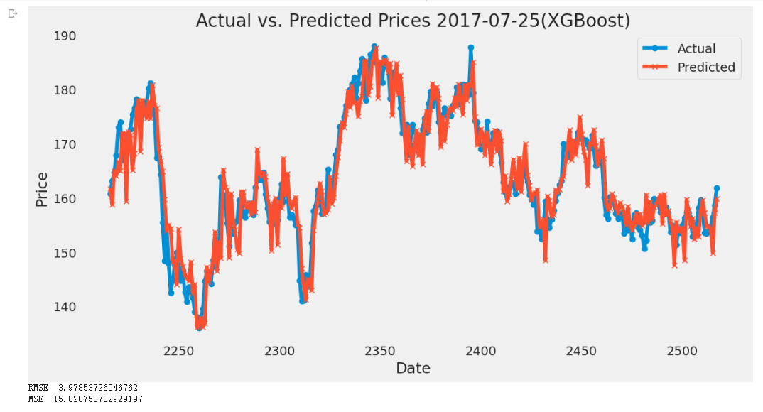
Figure 4: Plot of XGBoost Model of CVX from 2017-07-25 to 2023-07-25

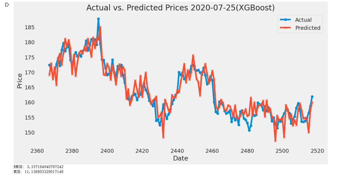
Figure 5: Plot of XGBoost Model of CVX from 2020-07-25 to 2023-07-25

As shown in the above figures, the peak of the actual price in the small-size dataset is slightly larger than the predicted price. As increasing the sample size to medium and large-size datasets, the actual price is still greater than the predicted prices and the difference among them does not seem to change a lot. Therefore, according to the figures, the gap between the predicted price and the actual price does not change large enough to be visible to the naked eye along with the time flow. The RMSE value of those years fluctuates between 3.3 to 3.9. It is not a large change compared to the stock prices (all prices are greater than 100 dollars and the prices wave between 140 to 180 dollars on most days). Therefore, the change in the dataset size does not make a significant impact on the accuracy of the prediction under XGBoost.

3.2. LSTM

Since the LSTM model easily causes overfitting problems, this paper initially did the data scaling for the dataset installed from Yahoo Finance. the data is normalized within the range [0,1] by using Min-Max scaling. Then, this paper splits it into training and testing subsets with an 80-20 split ratio. Also, the dropout layers are added to further prevent overfitting while defining the LSTM model. In the training part, this paper validated the model on the test data for 10 epochs with a batch size of 32. Then, the ModelCheckpoint is used to track the lowest MAPE on the validation data.

To analyze the final result, this paper plotted both the predicted data and actual data in the following Figures 6-8:

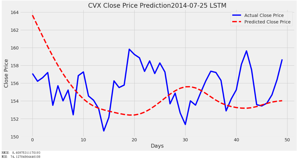
Figure 6: Plot of LSTM Model of CVX from 2014-07-25 to 2023-07-25

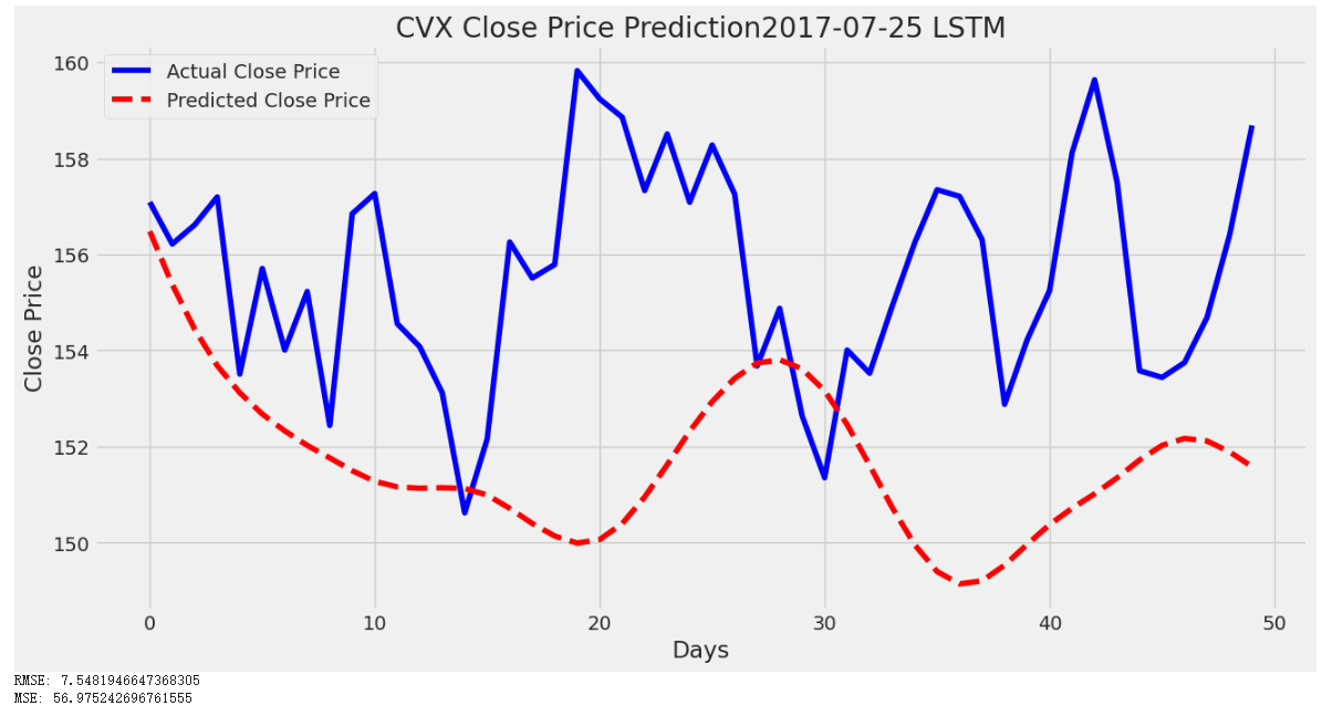
Figure 7: Plot of LSTM Model of CVX from 2017-07-25 to 2023-07-2

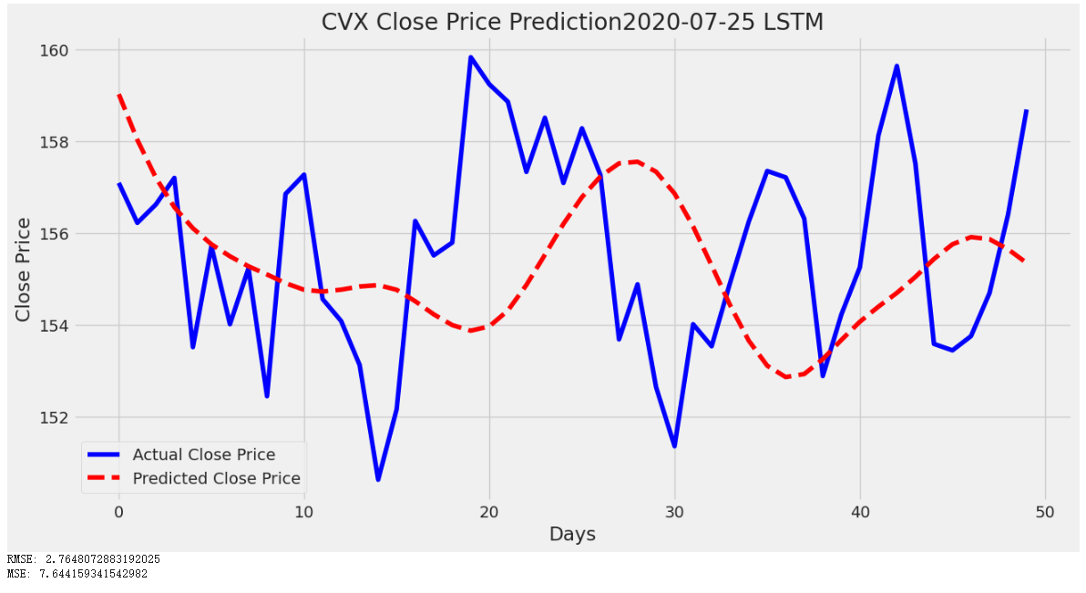
Figure 8: Plot of LSTM Model of CVX from 2020-07-25 to 2023-07-25

By comparing the predicted value and the actual value in the plot above, the gap among them has significantly changed along with the decreasing sample size.

In a large-size dataset, the predicted value started at around 164 dollars, but the actual price started at around 157 dollars. Also, the wave of the predicted price does not match the actual price well because the predicted price hits its bottom at the actual price’s peak.

In a medium-sized dataset, although the waves still do not match well the prediction is visually more consistent with the actual price. Also, at the peak of the actual price, the predicted price is the second lowest, which is an improvement.

In a small-size dataset, the figure experienced a significant improvement. The wave of predicted prices in the small-size dataset has a similar wave compared to the predicted prices in the medium-size dataset, but in the small-size dataset, the wave is overall shifted upward. Shifting the wave upward causes the predicted prices in a small-size dataset to fit better with the actual prices.

Also, the RMSE values would decrease as the dataset size decreases. The small-size dataset is the smallest dataset and has the lowest RMSE number. Having a smaller RMSE means having a more accurate predicted price. Thus, the LSTM model tends to generate more concise stock prices with small datasets.

3.3. Comparison

As shown in Table 1, the XGBoost model has better accuracy in the large and medium-size dataset, and LSTM model has better accuracy in the small-size dataset. XGBoost model does not have a tendency to increase RMSE value while increasing the dataset size. On the other hand, increasing the dataset size from small to medium to large tends to boost up the RMSE value.

Table 1: RMSE for XGBoost and LSTM

4. Conclusion

In conclusion, from the perspective of testifying the impact of dataset size on the accuracy of the models, the two models have distinct performances in different sizes of datasets. In the large and medium-size datasets, XGBoost has obviously less RMSE value compared to LSTM’s, representing XGBoost model has higher accuracy in large and medium-size. In the small-size dataset, the LSTM model is more accurate because it has less RMSE value than XGBoost. The LSTM model is easier to be impacted by the dataset size changes, representing that the LSTM model might encounter problems like overfitting in a large dataset. Also, in the small-size dataset, the LSTM model has higher prediction performance than XGBoost. Therefore, in the small-size dataset, using the LSTM model might result in a more accurate output compared to the XGBoost model. Other than that, using the XGBoost model might be a better decision because the XGBoost model performs a more stable prediction.

References

[1]. Chung, J., Gulcehre, C., Cho, K., and Bengio, Y. (2014). Empirical evaluation of gated recurrent neural networks on sequence modeling. arXiv preprint arXiv:1412.3555.
[2]. Kumar, D., Sarangi, P. K., and Verma, R. (2022). A systematic review of stock market prediction using machine learning and statistical techniques. Materials Today: Proceedings, 49, 3187-3191.
[3]. Friedman, J. H. (2001). Greedy function approximation: a gradient boosting machine. Annals of statistics, 1189-1232.
[4]. Chen, T., and Guestrin, C. (2016). Xgboost: A scalable tree boosting system. In Proceedings of the 22nd acm sigkdd international conference on knowledge discovery and data mining, 785-794.
[5]. Saud, A. S., and Shakya, S. (2020). Analysis of look back period for stock price prediction with RNN variants: A case study on banking sector of NEPSE. Procedia Computer Science, 167, 788-798.
[6]. Chudziak, A. (2023). Predictability of stock returns using neural networks: Elusive in the long term. Expert systems with applications, 213, 119203.
[7]. Hochreiter, S., and Schmidhuber, J. (1997). Long short-term memory. Neural computation, 9(8), 1735-1780.
[8]. Chen, Y., Wu, J., and Wu, Z. (2022). China’s commercial bank stock price prediction using a novel K-means-LSTM hybrid approach. Expert Systems with Applications, 202, 117370.
[9]. Bhandari, H. N., Rimal, B., Pokhrel, N. R., Rimal, R., Dahal, K. R., and Khatri, R. K. (2022). Predicting stock market index using LSTM. Machine Learning with Applications, 9, 100320.
[10]. Sak, H., Senior, A., & Beaufays, F. (2014). Long short-term memory based recurrent neural network architectures for large vocabulary speech recognition. arXiv preprint arXiv:1402.1128.
[11]. Luo, Y., Ye, W., Zhao, X., Pan, X., and Cao, Y. (2017). Classification of data from electronic nose using gradient tree boosting algorithm. Sensors, 17(10), 2376.
Cite this article
Li,Z. (2023). Comparison of XGBoost and LSTM Models for Stock Price Prediction. Advances in Economics, Management and Political Sciences,61,147-155.
Data availability
The datasets used and/or analyzed during the current study will be available from the authors upon reasonable request.
Disclaimer/Publisher's Note
The statements, opinions and data contained in all publications are solely those of the individual author(s) and contributor(s) and not of EWA Publishing and/or the editor(s). EWA Publishing and/or the editor(s) disclaim responsibility for any injury to people or property resulting from any ideas, methods, instructions or products referred to in the content.
About volume
Volume title: Proceedings of the 2nd International Conference on Financial Technology and Business Analysis
© 2024 by the author(s). Licensee EWA Publishing, Oxford, UK. This article is an open access article distributed under the terms and
conditions of the Creative Commons Attribution (CC BY) license. Authors who
publish this series agree to the following terms:
1. Authors retain copyright and grant the series right of first publication with the work simultaneously licensed under a Creative Commons
Attribution License that allows others to share the work with an acknowledgment of the work's authorship and initial publication in this
series.
2. Authors are able to enter into separate, additional contractual arrangements for the non-exclusive distribution of the series's published
version of the work (e.g., post it to an institutional repository or publish it in a book), with an acknowledgment of its initial
publication in this series.
3. Authors are permitted and encouraged to post their work online (e.g., in institutional repositories or on their website) prior to and
during the submission process, as it can lead to productive exchanges, as well as earlier and greater citation of published work (See
Open access policy for details).