1. Introduction

The concept of an investment portfolio entails the amalgamation of various assets, with the aim of diversifying risks associated with investments and attaining an optimal distribution of both risks and rewards. This approach is a viable strategy for investors and financial institutions to mitigate potential risks. Investors or financial institutions typically own a diverse range of assets within their investment portfolios, including but not limited to stocks, bonds, bank deposits, and real estate. In order to attain investment diversification, it is important to spread the risks associated with various assets, hence enhancing potential returns. Risk analysis in portfolio management involves the imperative to assess and evaluate the interplay between different assets within a portfolio, quantify diverse risks, and establish a foundation and framework for the investment composition of said portfolio. Investors engage in market participation with the objective of acquiring supplementary advantages. Nevertheless, after an investment is initiated in the market, it does not automatically provide a return, and there exists a potential for financial loss in the market. Hence, the establishment of a diversified portfolio serves as a reliable strategy for investors to mitigate potential market fluctuations and secure profitable returns. In order to effectively evaluate a portfolio, it is important to assess and quantify diverse risks, conduct a comprehensive analysis of the entire risk profile, and carefully consider the inclusion of both high-risk and risk-free assets. In order to ensure safety, it is important to possess a collection of assets that are devoid of any risk. In order to generate financial gains, it is necessary to possess a collection of high-risk investments. Consequently, the investment portfolio has the capacity to formulate investment strategies based on the investor’s risk tolerance and the attributes of the asset portfolio.

Given the inherent uncertainty and dynamic nature of the financial market, it is imperative for investors to adapt and optimize their portfolios in response to market fluctuations. This proactive approach serves to mitigate risks and enhance potential returns. Hence, this study will employ a literature review methodology to comprehensively examine portfolio optimization and risk analysis, aiming to enhance investors’ ability to effectively manage investment risks and achieve superior returns. Furthermore, the scholarly investigation into portfolio optimization and risk analysis inside financial markets can furnish investors with a solid empirical foundation for their decision-making processes. By means of analyzing and constructing a scientific portfolio optimization model and parallel algorithm, investors are able to enhance the precision of estimating portfolio returns and risks, and subsequently optimize their investment strategies accordingly. This will aid investors in making more educated investment selections, hence enhancing success rates and investment returns.

2. Portfolio optimum

2.1. Definition and objectives of the portfolio

An investment portfolio, alternatively referred to as an asset portfolio, encompasses a collection of diverse financial assets, including but not limited to stocks, bonds, and cash. The focal points of this study encompass equities, bonds, foreign exchange, options, precious metals, financial derivatives, real estate, land, as well as assets including antiques, listed business status, art, and wine. The objective is to construct an asset portfolio that possesses optimal attributes such as enhanced liquidity, stability, high returns, and minimal investment risk. Portfolios can be effectively managed by a range of stakeholders, including individual investors, financial professionals, hedge funds, banks, and various other financial institutions. However, it is important to note that the portfolio will not encompass consumer goods such as sports cars, televisions, cosmetics, apparel, and similar items. This exclusion is mostly due to their lack of potential for appreciation, or in certain cases, their potential for depreciation.

2.2. Composition and type of investment portfolio

Portfolios vary widely. Generally, the market portfolio is used more. The market portfolio includes well-known asset classes like equities, real estate, and bonds. Portfolio diversification is carefully combining market assets in specified amounts to maximize investment returns. Market portfolios help investors allocate their portfolios, reducing risk and increasing returns. Minimum variance, tangential, and efficient frontier portfolios are three ways to build an efficient market portfolio. Investors can maximize returns and minimize capital market risks by making sensible capital allocation and risk management decisions. The “least variance portfolio” has the lowest investment risk in a given market. This metric is suitable for low-risk investors because it depends on each asset’s weight and covariance matrix. The relationship between risk and return is fair, with low risk resulting in lower returns. Tangent portfolios strike the best market-specific balance between return and risk. By strategically allocating market portfolio investments, optimal investment results can be achieved. Tangent portfolios are suitable for investors that are willing to take more risks for larger gains. The effective frontier portfolio includes tangent investment portfolios. Investors can also choose efficient frontier portfolios based on their risk choices and rewards.

2.3. The theoretical basis of portfolio optimization

In 1952, American economist Markowitz published “Portfolio Selection” and introduced the portfolio theory. A mean-variance model helps the person balance portfolio risks and rewards. After that, they proposed a fundamental approach for choosing the best portfolio based on asset correlation. The decision-making references in this resource help financial institutions and investors manage risks and boost investment returns. This approach makes financial investment decision-making more scientific and reasonable, improving financial industry efficiency. In Yang Ming’s scholarly article, which is grounded in Markowitz’s model, the author presents the subsequent hypothesis [1]:

1. Investors are risk averse, whose goal is to pursue higher investment return with the same investment risk, or to pursue lower investment risk with the same investment return.

2. Investors make decisions based on expected return and return variance. Higher investment risk requires additional investment returns to compensate.

3. The investment period is a single period, and shorting assets is not allowed.

4. Capital markets are efficient, and the prices of securities reflect their intrinsic values. Any information about a security is available to every investor in the market in a timely manner.

5. Every security in the capital market is infinitely divisible. This means that investors can buy less than one share of the security.

6. The capital market has sufficient supply elasticity for individual investors, that is, the buying and selling of any securities in the portfolio will not affect the market price.

The paper uses Markowitz’s assumption-based mean-variance model. This model shows a compilation of models that find portfolios that maximize returns and minimize risk at a given risk. The ideal portfolio asset allocation and risk-return profile can be calculated using this equation. The idea is that a multi-asset portfolio can reduce single-asset investing risks. Diversifying assets among investment vehicles lowers investment differentials. Investment variance can illustrate that portfolio diversification reduces variance even if the two asset portfolios are strongly correlated. Two perfectly negative-correlated assets have the lowest portfolio variance. A perfect positive correlation has a correlation coefficient of 1. A gain in one asset increases another, while a reduction in one diminishes another. For perfect negative correlation, the correlation coefficient is -1. When one object grows in value, the other declines. When one asset falls, another rises. Thus, when assets have less than perfect positive correlation, many high-risk portfolios have lower total risk than their component dangers. A perfect negative correlation with other investments that fluctuate similarly reduces the portfolio’s variance to zero, allowing the investor to maximum returns.

2.4. Methods and models for portfolio optimization

This paper presents a portfolio optimization model and conducts an empirical examination of uncorrelated assets, drawing on the research conducted by Lin Chunyan [2]. Utilize the Markowitz portfolio optimization model presented herein to identify a portfolio exhibiting elevated investment efficiency.

\( min({σ^{2}}=\sum _{i=1}^{n}σ_{i}^{2}x_{i}^{2} +\sum _{ \begin{array}{c} i, j=1 \\ i≠1 \end{array} }{σ_{ij}}{x_{i}}{x_{j}}) \)

\( s.t\sum _{i=1}^{n}{x_{i}}{r_{i}}=r, \sum _{i=1}^{n}{x_{i}}=1 \)

In the computation, it is imperative to approximate the covariance between the i-th and j-th rates of return of a risky asset, denoted as σij, as well as the expected rate of return, ri, for each individual risky asset. A positive value of σij indicates that the realized return of one asset exceeds its projected return, and the same holds true for the other asset. A negative value of σij signifies that the realized return of the asset surpasses the anticipated return. In contrast, the realized return on alternative assets is lower than the anticipated return. The value of \( {σ_{ij}} \) is determined to be 0, which signifies that there is no correlation between assets and revenue/profit. In academic terms, these assets are referred to as irrelevant assets. Upon careful examination of the provided formula, it becomes evident that the act of merging assets that exhibit no correlation can effectively mitigate risk, while leaving the actual returns unaffected. As previously mentioned by the author in the preceding chapter of this research, it has been asserted that investors can optimize portfolio performance by seeking negative correlation. However, it is important to note that in practice, real returns frequently exhibit divergent trends even in the presence of negative correlation. This phenomenon poses a challenge to the construction of portfolios aimed at achieving higher real returns. When investors select a portfolio, they have the option to include various types of assets, such as stocks and bonds, which are distinct from one another.

3. Risk Analysis

3.1. Definition and classification of risk and risk measurement index

Liu Yanchun’s work reviews risk definitions [3], focusing on two major factors. Risk is the likelihood and severity of undesirable consequences. The initial likelihood, potential magnitude, and overall probability of a bad outcome are all aspects of risk. Risk is caused by the interaction of risk events, consequences, and variables. Risk encompasses these fundamentals. Multiple major financial risk categories exist. Market risk—losses from asset market price swings, both up and down—is a major risk. System breakdowns and worker errors cause financial loss, the second operational risk. Third, credit risk—economic damages from a party’s failure to satisfy financial obligations—is important. Losing money if a contract is improperly completed or finalized is the fourth legal risk. This generally implies credit risk. Financial losses from asset purchases and sales in a market that don’t meet expectations or can’t be converted into cash are liquidity risk.

The subsequent tools are frequently utilized for the quantification and assessment of risk. Volatility refers to the extent of fluctuations in asset prices. A decrease in volatility corresponds to a decrease in price volatility, resulting in a reduction in risk. Furthermore, beta serves as an indicator of the level of volatility exhibited by a portfolio or stock in relation to the broader market. When the beta coefficient is negative, it indicates that the stock exhibits lower volatility and risk compared to the overall market. Conversely, in cases when the beta coefficient exceeds 1, the level of risk will be elevated.

3.2. Risk analysis methods and models

Finance has complexified asset arrangements, according to Liu Yanchun. Thus, some financial market risk measurement approaches are inadequate [3]. To quantify market risk, he developed Var. A person estimated an asset portfolio’s maximum loss over a future timeframe assuming average market swings. A confidence level and holding duration are needed to make any variable value relevant. Individuals’ confidence in a conclusion or opinion is called confidence level. It also denotes the proportion of sample intervals that contain the overall parameter while creating it, commonly represented as. During the holding phase, VaR is calculated. The holding period depends on market liquidity. Fast-liquidity trading positions may benefit from a shorter holding period than slow-liquidity ones. Prerequisite data is needed to calculate variance. Thus, shorter holding durations enable more early data collection. Choose a confidence level based on scenario and goals. When data is scarce, investors that prioritize computation accuracy may gain from decreased confidence. When calculating internal risk capital using Value at Risk (VaR), security and confidence are positively connected. Our discussion will introduce two non-parametric VaR risk measurement methodologies. Historical simulation takes lots of data. If the income distribution remains stable during the designated period, a historical trend reversal will inflict a less severe unanticipated loss than the sample. The formula is:

\( R_{t}^{P}=\sum _{i=1}^{m}{w_{i}}{R_{it}}, t=1,2,...,T \)

The variable “ \( {R_{it}} \) ” represents the profit and loss of asset i at time t. “ \( {w_{i}} \) ” denotes the investment proportion of asset i. “m” represents the number of investment assets in the portfolio. Lastly, “T” refers to the historical profit and loss information over the past T days. The algorithm yields a chronological arrangement of historical profit and loss values, ranging from least to greatest. By utilizing the provided empirical distribution function, VaR values can be approximated at various confidence levels. The second method under consideration is the Monte Carlo simulation, which has the capability to generate a substantial number of scenarios and is deemed to be more precise compared to the preceding historical simulation approach. Nevertheless, if the resultant data sequence is a pseudorandom number, it will lead to inaccurate outcomes. The calculation procedure involves initially formulating a model that describes the dynamic progression of risk components. Subsequently, the error term is randomly simulated and subsequently substituted into the model containing the risk factors. By solving this modified model, the value of the risk can be determined.

4. Combination of portfolio optimization and risk analysis

4.1. Risk constraints of portfolio optimization

This section provides an overview of portfolio optimization techniques that incorporate risk limitations. Initially, it is important to note that the Value at Risk (VaR) metric, when applied within the context of risk limits, does not permit the practice of short selling. In a broad sense, the inclusion of short selling in the investment process amplifies the level of risk inherent in financial markets and poses potential challenges for investors. Hence, it is a common practice to prohibit short selling in nascent markets, such as the Chinese stock market. Hence, building off Zhang Peng’s research [4], this study aims to present an extended analysis of the mean-variance combination optimization approach using Value at Risk (VaR) values within the framework of a risk constraint that prohibits short selling. The model can be described as follows:

\( min {x^{T}}Gx/2 \)

\( s.t.\begin{cases} \begin{array}{c} {r^{T}}x≫{r_{0}} \\ {r^{T}}x≫{∅^{-1}}(c)\sqrt[]{{x^{T}}Gx}-{V_{a}}{R_{0}} \\ {e^{T}}x=1; x≫0 \end{array} \end{cases} \)

The model does not incorporate transaction costs and taxes, while making the assumption that the portfolio only consists of risky assets and that these assets are endlessly divisible. The present model enables us to examine the optimal allocation of assets for investors with the aim of minimizing portfolio variance, hence mitigating risk. Additionally, this model offers valuable references for investors seeking guidance in this matter. Based on Zhang Peng’s research, the analysis of six weighted stocks on the Shanghai Stock Exchange reveals the incorporation of VaR constraints into the mean-variance model. This integration aims to mitigate potential investment losses to a tolerable extent for investors by eliminating portfolios that are not preferred by investors. Nevertheless, the implementation of this limitation has concurrently diminished the array of choices available to investors.

4.2. Comprehensive methods and models for portfolio optimization and risk analysis

This section aims to present a comprehensive and precise overview of the models utilized in portfolio optimization and risk analysis, as discussed in Zhang Xifan’s scholarly study [5]. The author of the research also presented additional asset portfolio models that aim to minimize variance, drawing upon theories such as Markowitz’s.

\( \begin{cases} \begin{array}{c} minσ_{p}^{2}={Z^{T}}MZ \\ constraint condition{Q^{T}}Z=x1+x2+...+xn=1 \\ E({R_{P}})=E(k{)^{T}}∙Z=μ \end{array} \end{cases} \)

The expected rate of return for the determination is \( μ \) . Select the weight of the asset portfolio \( Z=(x1, X2, ......, Xn), \) T-square minimizes its total risk. The following are some model that provides expected return on investment and risk estimation. To calculate the expected return on investment of a certain security in the near future, local integral means need to be used to obtain the valuation model of the return.

\( E(k)=\frac{\sum _{i=1}^{m}{\overline{r}_{i}}}{m} \)

Based on the aforementioned classifications of risks delineated within this paper, it is also possible to categorize risks into two distinct categories: non-systematic risks and systematic risks. Non-systemic risk can be effectively mitigated by diversifying investment portfolios, however systemic risk is an intrinsic characteristic of the capital market and is not susceptible to dispersion through investment portfolios due to its association with global variables. Risk refers to the extent to which the anticipated future return on securities can fluctuate. Hence, the utilization of the variance of securities return as a risk metric is applicable inside investment portfolios. The proposed framework for assessing risk through the utilization of sample values derived from securities returns is as follows:

\( {σ^{2}}=\frac{1}{m-1}\sum _{i=1}^{m}[{\overline{r}_{i}}E(k){]^{2}} \)

The expected return model for each security was obtained later.

\( E({R_{i}})=\frac{\sum _{j=1}^{m}{\overline{r}_{ij}}}{m} \)

Which can be write as \( {σ_{ij}}={_\overline{m}^1}-1\sum _{k=1}^{m}({\overline{r}_{ir}}-E({R_{i}}) ({r_{jk}}-E({R_{j}})) \)

The symbol \( {σ_{ij}} \) represents the estimated covariance between the \( i-th \) security and the \( j-th \) security. By employing the aforementioned portfolio optimization technique discussed previously in this paragraph. Given specific projected return conditions, the objective is to determine the optimal weight allocation for an investment portfolio in order to minimize investment risks. Provide an additional constraint while considering a specific risk simultaneously. The model that attains the highest rate of return is outlined as follows:

\( max{R_{P}}={R^{T}}Z \)

\( σ_{P}^{2}={Z^{T}}MZ=σ_{0}^{2} \)

\( {Q^{T}}Z=x1+x2+...+xn=1 \)

4.3. Portfolio optimization and risk analysis in Chinese stock market

This part will utilize the aforementioned information to conduct empirical analysis and risk measurement of portfolio optimization. It aims to examine the validity and applicability of the aforementioned model in the context of real securities. According to the research conducted by Ni Yaoqi (2016), the concept of conditional value at risk (CVaR) serves as an enhanced and refined approach to the previously discussed value at risk (VaR) method. Conditional Value-at-Risk (CVaR) is a quantitative measure that represents the anticipated loss experienced by investors when the Value-at-Risk (VaR) threshold is surpassed within a certain level of confidence and time horizon. The mathematical expression for CVaR is as follows:

\( CVa{R_{a}}=E(X/X≫Va{R_{a}}) \)

For quantifying extreme value risk, CVaR is more thorough than VaR. Conditional Value at Risk (CVaR) must exceed VaR at the confidence level to meet the condition. Conditional Value at Risk (CVaR) highlights excessive tail losses and evaluates tail risk using expected values. This procedure yields more accurate and dependable measurements. These conclusions and approaches work effectively in the stock market, especially with increase and fall limitations. When confidence reaches 99%, CVaR and VaR comparisons between A and H shares become less important. According to the sources, investment portfolios must be objectively analyzed using Ni Yaoqi’s discoveries and preceding theories and models. The Shanghai and Shenzhen stock exchanges’ 300 component equities include 251 non-financial stocks listed for at least two years. These non-financial stocks were chosen since their stock price cycles may be incomplete and lack 24-month BETA value and volatility data. The multi-factor methodology sorts 251 stocks by factor value from 12 distinct variables. Annual average return and correlation coefficient between overall factor and return rate for the top 50 combinations are discovered. The differential return is calculated by comparing the last 50 combinations. The results are in Table 1.

Table 1: Statistical Results of Candidate Factors in Multifactor Model [6]

In order to account for the varying sizes and scales of different factors, it is imperative to standardize the scores of these factors. For instance, Zx1 denotes the standardized X1. Subsequently, the correlation test enables the examination of the correlation between the factors as well as the correlation between the factors and the income rate, as presented in Table 2.

Table 2: Correlation between various standardized factors and annual growth rate [6]

The next step is to use correlation and score each stock according to the following formula: \( Y1 = β1ZX1 + β2ZX2 + β3ZX3 + β4ZX4 + β5ZX5 + β6ZX6. \) The correlation coefficient Bx represents the relationship between the standardized factor x and the annual increase. The objective of this study is to assess the relative performance of 251 stocks and thereafter identify the stocks exhibiting promise for future growth based on a multi-factor quantitative stock selection methodology. The next step involves the selection of a portfolio consisting of the top 10 stocks, with the aim of assessing the efficacy of this selection based on the presence of any excess returns. According to the multi-factor model of stock selection, the portfolio generated a return of 119.62% within the corresponding time frame. Simultaneously, it is evident that the combination of these factors yields an effective excess rate of return of 15.29%. The subsequent phase involves doing an analysis of the aggregate returns of the portfolio in order to obtain a more comprehensible perspective. Given an initial asset of one unit, the price series of ten constituent stocks is transformed into a return series. The return series is then constructed using the same weight weighting, as depicted in Figure 1.

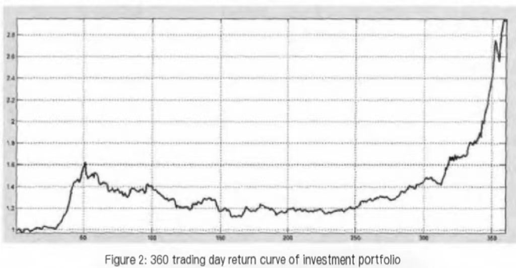
Figure 1: 360 trading day return curve of investment portfolio [6]

Subsequently, a risk analysis of the portfolio will be conducted. Once the daily return data for the entire portfolio has been acquired, it will undergo further analysis. This concept pertains to the maximum retracement, which refers to the displacement of the return on a chosen portfolio within a specified time period, commencing from a designated point in time. The extent of retracement, measured from the highest point to the lowest point, serves as an indicator of the potential maximum loss incurred by an investor subsequent to the purchase of the product. In Ni Yaoqi’s study, statistical procedures were conducted using the MATLAB program, leading to the identification of a maximum backtracking proportion of 30.71%. This implies that if an investor constructs a portfolio on the 51st trading day, they will encounter a loss of 30.71% until the 162nd trading day. Furthermore, it is important to acknowledge that the maximum retracement of losses seen in the past may also be encountered in future scenarios. In the context of hedge funds and quantitative strategy trading, the assessment of risk is a crucial consideration. Within this framework, the measure of maximum retracement assumes a significant role, surpassing the significance of volatility. The value at risk is calculated by using the portfolio yield distribution data. Here, CVaR for N days is calculated as NDays’ \( CVaR = One day \prime s CVaR × √N \) The next step is portfolio optimization for CVaR. Especially in China’s stock market, CVaR has a better ability to measure risks, reflecting tail risks, while variance reflects the overall up and down risk. The mean-cVAR model here is:

\( \begin{cases} \begin{array}{c} minCVa{R_{a}} \\ s.t.\sum _{i=1}^{n}{x_{i}}{r_{i}}=C \\ \sum _{i=1}^{n}{x_{i}}=1, i∈{N^{+}} \end{array} \end{cases} \)

Returning to the practical implementation, the analysis focuses on the return series of ten stocks over a period of 359 trading days. Subsequently, the best portfolio weight ratio is computed based on a predetermined risk value. Based on the analysis of the chosen stocks, it is evident that while the multi-factor model screening indicates a certain stock’s potential for upward movement, its overall trend is noticeably weaker compared to other stocks. Subsequently, following the use of the mean-CVAR model for optimization, it has been determined that the distribution of the five portfolios across their respective stocks approaches zero, indicating a significant enhancement in portfolio performance.

5. Limitations and future development of portfolio optimization and risk analysis

Methodology for risk assessment in practice, VaR has two drawbacks. Yang Shijuan’s article states that Value at Risk (VaR) is inconsistent since it fails sub-additivity [7]. Second, Var’s tail loss measurement is inadequate. It only tests sub-points within a certain confidence level, making the information below them untestable. These constraints make people ignore the minimal risk of major losses. In the last chapter, we introduced Conditional Value at Risk (CVaR) as an upgraded VaR technique. We believe the model lacks robustness due to CVaR’s sub-additivity. We believe VaR is stronger than CVaR. Therefore, some experts propose that considering both techniques together can be beneficial in practical implementation because they have complimentary capabilities. In his research essay, Li Hui argues that the Markowitz securities investing model’s assumptions are too strict in real-world circumstances, making its existence unlikely. Investors’ usage of the Markowitz securities investment model is highly limited. By being more flexible with conditional assumptions, investors can better understand and use market dynamics. The current model also ignores key securities trading expenditures, particularly for frequent, short-term traders seeking huge profits. Transaction costs may rise due to frequent stock trading and other variables. Omitting transaction charges, which often lead to portfolio management and investing failure, can have serious consequences [8].

6. Conclusion

This study is centered around Markowitz’s portfolio optimization model, which is utilized to introduce the notion of unrelated assets as a point of reference for investors’ investment portfolios. Subsequently, two primary approaches for assessing risk, namely Value at Risk (VaR) and Conditional Value at Risk (CVaR), were introduced, accompanied by the presentation of their respective models. Ultimately, through the utilization of the well-established mean CVaR model, an empirical analysis was conducted on the Chinese stock market, resulting in the acquisition of an optimum investment portfolio.The scope of research in this work is limited, focusing solely on the analysis and description of empirical methodologies employed for a selection of representative stocks in China. Consequently, the findings may not be universally applicable to stock markets in all countries or specific stock markets under unique circumstances. In subsequent investigations, it is recommended that additional empirical examination be undertaken pertaining to the stock markets of diverse nations, with a simultaneous exploration of the suitability and constraints inherent in the employed methodologies and models.

References

[1]. Yang Ming. Research on Portfolio Optimization of Individual Investors in China at Present Stage [D]. Fudan University, 2009:12 - 14.
[2]. Lin Chunyan. Portfolio optimization in multiple environments and its application [D]. Dalian University of Technology, 2004: 15 - 16.
[3]. Liu Yanchun. Research on Measurement and portfolio optimization of VaR in securities investment [D]. Northeastern University,2006:13 - 17,37 - 42.
[4]. Zhang Peng. Mean-variance portfolio optimization with no short selling based on VaR constraints [J]. Journal of Wuhan University of Science and Technology,2012,35(01):73-76.
[5]. Zhang Xifan, Li Xianxi, Shan Feng et al. Optimal selection of investment portfolio: Return and Risk Analysis [J]. Journal of Shenyang Institute of Aeronautical Technology,2001(02):81-83.
[6]. Ni Yaoqi. Empirical Analysis of CVaR risk Measurement and portfolio Optimization [J]. Time Finance,2015(24):258-262+265.
[7]. Yang Shijuan. Calculation and empirical analysis of VaR and CVaR based on IS [D]. Guangxi Normal University,2015: 1 - 2.
[8]. Li hui. The markowitz portfolio model based on transaction cost correction [J]. Modern commercial and trade industry, 2010, 22 (18) : 16-17. DOI: 10.19311 / j.carol carroll nki. 1672-3198.2010.18.009.
Cite this article
Li,G. (2023). Portfolio Optimization and Risk Analysis in Financial Markets. Advances in Economics, Management and Political Sciences,61,236-246.
Data availability
The datasets used and/or analyzed during the current study will be available from the authors upon reasonable request.
Disclaimer/Publisher's Note
The statements, opinions and data contained in all publications are solely those of the individual author(s) and contributor(s) and not of EWA Publishing and/or the editor(s). EWA Publishing and/or the editor(s) disclaim responsibility for any injury to people or property resulting from any ideas, methods, instructions or products referred to in the content.
About volume
Volume title: Proceedings of the 2nd International Conference on Financial Technology and Business Analysis
© 2024 by the author(s). Licensee EWA Publishing, Oxford, UK. This article is an open access article distributed under the terms and
conditions of the Creative Commons Attribution (CC BY) license. Authors who
publish this series agree to the following terms:
1. Authors retain copyright and grant the series right of first publication with the work simultaneously licensed under a Creative Commons
Attribution License that allows others to share the work with an acknowledgment of the work's authorship and initial publication in this
series.
2. Authors are able to enter into separate, additional contractual arrangements for the non-exclusive distribution of the series's published
version of the work (e.g., post it to an institutional repository or publish it in a book), with an acknowledgment of its initial
publication in this series.
3. Authors are permitted and encouraged to post their work online (e.g., in institutional repositories or on their website) prior to and
during the submission process, as it can lead to productive exchanges, as well as earlier and greater citation of published work (See
Open access policy for details).