1. Introduction

Gross Domestic Product (GDP) is the final result of the production activities of all resident units in a country (or region) over a certain period of time. It is worth noting that GDP is a significant used to measure the economic condition of a country [1]. Establishing a scientific and reasonable prediction model to quantitatively analyze and predict the factors that affect the GDP can not only infer the overall development of the economy, but also provide rational policy suggestions for relevant departments.

This paper will address the economic growth models of the strongest province in northern China (Shandong Province) and the strongest province in southern China (Guangdong Province) in China via different linear regression models, and compare their respective important economic growth factors, which will help in-depth understanding of the economic development characteristics and government intervention measures in different regions of China, and promote the coordinated development of regional economy and win-win cooperation. Someone find that there is a long-term stable co-integration relationship between fiscal revenue and expenditure and GDP [2]. For example, in the short run, there is a dynamic adjustment mechanism between GDP and fiscal balance, and in the long run, GDP and fiscal balance are highly statistically correlated. Multiple linear regression models can not only achieve dynamic fitting, but also quantitatively investigate the correlation between variables. In addition, GDP is dependent on most economic factors, and basically does not saturate with the development of industries. This indicates that multiple linear regression is suitable for related research of GDP. One more step should be made in this paper is to compare the differences in economic factors affecting GDP between regions. The main economic factors affecting Guangdong's GDP are secondary industry, foreign investment and urbanization [3], while the main economic factors affecting Hebei's GDP are employment population, fixed assets and fiscal revenue [4]. Therefore, there are differences in the main economic factors that affect the GDP of the northern and southern regions. It would be helpful for us if we can identify the economic development advantages of northern and southern regions.

The following structure of this paper will contain a short literature review of previous works. And then this paper will discuss the linear regression-based GDP economic growth model. To further investigate the relationship between GDP growth and regions, the next step will be to separately discuss the main economic factors related to GDP in the northern and southern provinces. Last, a short conclusion will be made.

2. Previous works

Accurate forecasting of regional or national GDP is of great significance for guiding development. Much research has shown that the development trend of various economic indicators can be calculated based on statistical methods. Zheng et al. [5] argued that there is a linear correlation between the three industries and GDP growth. The tertiary industry is developing rapidly, and the industry has shown a downward trend in recent years. Jiang [6] based visual analysis and basic statistical data to predict the GDP per capital of each country through multiple linear regression. Bai [7] argued that household consumption level, total import and export trade, foreign direct investment and research and development expenditure are the four most important factors affecting China's GDP growth. Based on the study of GDP in different provinces, in Wu et al. 's work [3], Guangdong should improve the overall level of scientific and technological innovation in the secondary industry and drive GDP development with science and technology. Guan [8] implied that the secondary industry is the driving force to promote the GDP growth of Henan Province, but the proportion of the tertiary industry in the GDP of Henan Province is also increasing, indicating that the rapid development of the service industry needs to be increased in the future to greatly accelerate the GDP growth rate. Liang [9] investigated that the residents' consumption level, research and experimental development (R&D) expenditure, energy consumption, total import and export trade, and foreign direct investment are the five most important factors affecting the GDP growth of Anhui Province. Zhu [10] argued that the proportion of industry in the GDP of Anhui is high and has a growing trend, which has a direct and significant impact on the regional economy. There is a synergistic relationship between household consumption level and regional GDP, that is to say, household consumption has a greater role in promoting regional economic growth, and the increase of regional GDP will also stimulate consumption in the reverse direction. Wang [11] argued that the main reasons for the rapid economic development of Shandong Province are the retail sales of social consumer goods and the total volume of import and export trade. Shandong can not only expand the consumption strategy, but also maintain the steady growth of foreign trade. In Li’s work [12], the changes of employment, investment in fixed assets, fiscal revenue and price index are the main factors affecting Jiangsu's GDP, which show a positive correlation trend. It is necessary for the government to regulate financial revenue and expenditure, stabilize the relationship between the government and the market, and effectively promote the comprehensive, coordinated and sustainable development of Jiangsu Province's economy.

Moreover, methods that integrate multiple prediction models or time series also achieve high model accuracy. For example, Xue et al. [13] applied exponential smoothing method, ARIMA model and combined forecasting model to forecast Chongqing GDP respectively, and the results expound that the combined forecasting model has the highest accuracy. Based on the exponential smoothing method and regression analysis, Wang et al. [14] constructed a prediction model for the recent data of time series historical data and predicted China in 2017, which indicates that the method is feasible in the short- and medium-term prediction of data. Liu [15] applied univariate linear regression to predict the GDP of Gansu Province, and although the results were basically in line with the predicted value during the national 13th Five-Year Plan period, only a single variable was used to predict, and the model lacked complexity and could not really fit the data characteristics of GDP. Therefore, this paper proposed to apply multivariate linear regression to predict GDP.

3. Approach

3.1. Model building

There are many factors influencing GDP. After relevant literature research [2-12], a total of six independent variables related to GDP will be preliminarily screened from the two directions of residents' economic activities and industrial structure, and then relevant index data of Guangdong and Shandong from 2010 to 2021 are collected to establish the following multiple regression model:

\( Y={β_{0}}+{β_{1}}{X_{1}}+{β_{2}}{X_{2}}+{β_{3}}{X_{3}}+{β_{4}}{X_{4}}+{β_{5}}{X_{5}}+{β_{6}}{X_{6}}+ε \) (1)

In the regression model, \( Y \) to be explained variable, \( {X_{i}}(i=1,2,…,6) \) as explanatory variables, \( {β_{i}}(i=1,2,…,6) \) for the corresponding regression coefficient, \( {β_{0}} \) for regression constant, \( ε~N(0,{σ^{2}}) \) for random error.

3.2. Indicator screening

Based on the established multiple linear regression model, this institute selected variables are as follow.

(1) \( Y \) is GDP, which is a measure of the total amount of economic activity in a country or region.

(2) \( {X_{1}} \) is residents’ consumption level, which is mainly used to reflect the impact of residents’ consumption on GDP.

(3) \( {X_{2}} \) is urban employed population, which is mainly used to reflect the impact of labor market conditions on GDP.

(4) \( {X_{3}} \) is residents disposable income, which is mainly used to reflect the impact of residents' living standards on GDP.

(5) \( {X_{4}} \) is industrial added value, which is the added value created by the industrial sector in a time specific period. It is mainly used to reflect the impact of industrial development on GDP.

(6) \( {X_{5}} \) is the added value of the real estate industry, which is one of the significant components of the added value of the tertiary industry. It is mainly used to measure the impact of real estate industry on GDP.

(7) \( {X_{6}} \) is the value added of the primary industry, which mainly reflects the impact of the added value created by agriculture and resource industries on GDP.

Through the index detection of multiple linear regression, the main variable indicators that have a significant effect on GDP growth are identified, and then the regression equation is determined, and the prediction analysis is carried out. Based on the important economic indicators of Guangdong and Shandong, the similarities and differences of important economic indicators in the north and south provinces of China will be studied.

Table 1: Indicator screening table.

3.3. Data source

For the practicability of the research, the data of this research come from the National data website released by the National Bureau of Statistics (http://data.stats.gov.cn), and the data of various economic indicators from 2010 to 2021 are respectively collected and sorted into a format suitable for statistics.

4. Experimental Procedure

4.1. The construction of Guangdong GDP model

4.1.1. Correlation analysis

In this paper, IBM SPSS Statistics 23 software is used as the statistical analysis tool to import the data that conformed to the statistical format of the data. Make correlation analysis between dependent variable and independent variable to ensure that each independent variable has a regression effect on GDP. The Pearson correlation coefficient matrix obtained is as follows.

Table 2: Pearson correlation coefficient matrix (Guangdong)

From the correlation coefficient can see six independent variables is highly correlated with Guangdong’s GDP, and all through the Pearson correlation two-tailed test. Therefore, regression analysis can be performed on the above variables.

4.1.2. Parameter estimation

Based on model (1) and in order to obtain independent variables that have a significant impact on GDP, this research first uses stepwise regression method to estimate parameters. The method of stepwise regression is to introduce variables gradually. After each variable is introduced, the selected variables are tested one by one. When the originally introduced variable becomes no longer significant due to the introduction of subsequent variables, it is necessary to remove it. Each step of stepwise regression requires an F-test to ensure that the final regression subset is the optimal regression subset. The parameters obtained by stepwise regression are as follows.

Table 3: Stepwise regression coefficient table (Guangdong).

Table 4: Primary model summary table (Guangdong).

According to the preliminary regression results, the multiple regression model is obtained as follows:

\( Y=-1803.046-0.328{X_{1}}+0.956{X_{3}}+1.441{X_{4}}+2.578{X_{5}} \) (2)

4.1.3. Model test

4.1.3.1. Statistical result testing

From the multiple regression model obtained above, it can be seen that \( {R^{2}} \) =1.0000, and the adjusted coefficient of determination is \( {\bar{R}^{2}} \) =1.000, indicating that the regression model has a remarkably high degree of fit to the sample. When performing the F-test, the null hypothesis \( {H_{0}} \) is: \( {β_{1}}={β_{3}}={β_{4}}={β_{5}}=0 \) . At the specified significance level α=0.05, the p-value corresponding to the F-test is less than 0.05, so the null hypothesis \( {H_{0}} \) should be rejected. It means that residents' consumption level \( {X_{1}} \) , residents' disposable income \( {X_{3}} \) , industrial added value \( {X_{4}} \) and the added value of real estate industry \( {X_{5}} \) combined have a significant impact on Guangdong’s GDP growth. The t-test result indicates that their individual regression effect on Guangdong's GDP is also significant.

4.1.3.2. Multicollinearity test

Multicollinearity phenomenon in multiple linear regression model is frequently. If the correlation between independent variables exceeds the correlation between independent variables and dependent variables, the resulting multiple linear regression model will lose its stability and lead to the appearance of regression coefficients that are not economically meaningful. For example, residents’ consumption level should play a role in promoting GDP, but its corresponding regression coefficient (-0.328) is negative. Therefore, it is necessary to perform multicollinearity test on all independent variables. Variance inflation factor (VIF) is often used to judge multicollinearity problems. The larger the VIF, the more serious the multicollinearity between the independent variables. It is recognized that when VIF \( \gt \) 10, it indicates that the multicollinearity problem among independent variables will seriously affect the accuracy of model estimation. The result of multicollinearity test implies that the VIF of \( {X_{1}} \) , \( {X_{3}} \) , \( {X_{4}} \) and \( {X_{5}} \) are 173.749, 51.043,90.135 and 5.584 respectively, which indicating that the model has serious multicollinearity problems. In the next step, the model will be modified according to the problem that multicollinearity so as to ensure that the multicollinearity will no longer appear in the new model, so that the regression results obtained are more reliable and of practical significance.

4.1.4. Model modification

4.1.4.1. Ridge regression

In order to solve the problem that the effect of ordinary least squares method becomes worse due to multicollinearity, the ridge regression method was first proposed by Goole in 1962 and discussed in detail in 1970 [16]. Before introducing ridge regression, the design matrix \( X \) and the identity matrix \( I \) need to be introduced in this chapter. When there is multicollinearity between the independent variables, the design matrix \( X \) is ill-conditioned, that is to say, \( det⁡({X^{ \prime }}X) \) is very close to zero such that its inverse matrix is very sensitive to affect stability, where \( X \prime \) represents the transpose of \( X \) . Adding a normal number matrix \( kI(k \gt 0) \) to \( {X^{ \prime }}X \) , then \( {X^{ \prime }}X+kI \) is much less close to singularity than \( {X^{ \prime }}X \) is to singularity. It is common to define \( \hat{β}(k)={{(X^{ \prime }}X+kI)^{-1}}X \prime y \) as the ridge regression estimate of \( β \) .

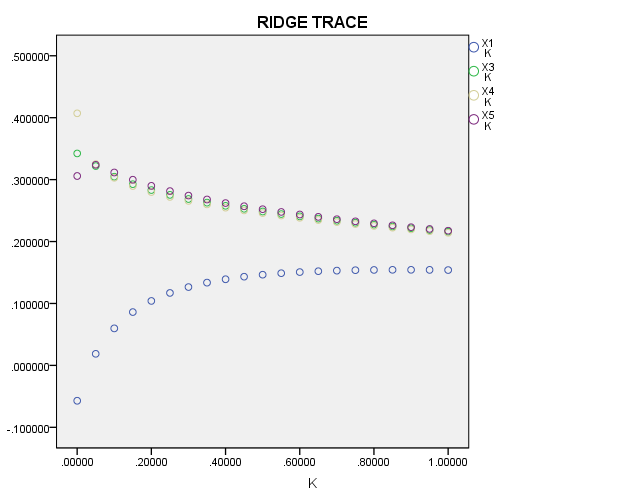
Figure 1: Ridge trace of \( {X_{1}} \) , \( {X_{3}} \) , \( {X_{4}} \) and \( {X_{5}} \) (Guangdong).

In Figure 1, when \( k \) increases slightly from \( 0 \) , \( {\hat{β}_{1}}(k) \) rises significantly and tends to \( 0 \) rapidly, thus losing the ability to predict. From the perspective of the ridge regression, \( {X_{1}} \) does not play an important role in \( y \) , and this variable can be eliminated.

4.1.4.2. Modified model

After eliminating the independent variable \( {X_{1}} \) , it indicates that when the ridge parameter \( k \) changes within \( (0,0.2) \) , the ridge traces of the other independent variables are basically stable. By \( {R^{2}} \) and equation significance comparison, it is found that when \( k=0.14 \) , the ridge regression model is optimal, and the parameters are as follows:

Table 5: Ridge regression coefficient table (Guangdong).

Table 6: Model summary table (Guangdong).

The ridge regression equation can be obtained from Table 5 as follows:

\( Y=-2801.887+0.919{X_{3}}+1.211{X_{4}}+2.756{X_{5}} \) (3)

(3) indicates that when other conditions remain unchanged, residents' disposable income increases by 1 yuan, Guangdong's GDP increases by an average of 0.919 billion yuan. When other conditions remain unchanged, each increase in industrial added value of 1 billion yuan will increase Guangdong's GDP by 1.211 billion yuan on average. When other conditions remain unchanged, the added value of real estate industry increases by 1 billion yuan, and Guangdong's GDP increases by 2.756 billion yuan on average.

4.1.5. Model prediction effect analysis

Based on model (3), residents' disposable income, industrial added value and the added value of real estate industry are taken as independent variables. The predicted GDP of Guangdong from 2010 to 2022 is calculated and compared with the real value. The fitting effect will be tested by relative error in this research. Relative error ( \( δ \) ) is the ratio of absolute error to the true value multiplied by 100%, which can more intuitively understand the difference between the predicted value and the true value, which is helpful to evaluate the accuracy of the prediction model. The results show that the \( δ \) of the predicted and the real value in each year is all within 2%, and the mean and median of \( δ \) are about 0.7%, indicating that the predicted GDP is very close to the real value, indicating that the model has a good degree of fitting. It has general applicability. the above data show that residents' disposable income, industrial added value and the added value of real estate industry are three important factors for Guangdong's GDP growth. The model fitting figure is as follows.

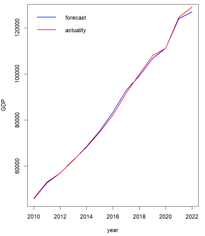
Figure 2: Model fitting figure (Guangdong).

4.2. The construction of Shandong GDP mode

From the correlation coefficient can see six independent variables is highly correlated with Shandong’s GDP, and all through the Pearson correlation two-tailed test. Therefore, regression analysis can be performed on the above variables.

4.2.1. Correlation analysis

Table 7: Pearson correlation coefficient matrix (Shandong).

4.2.2. Parameter estimation

The parameters obtained by stepwise regression are as follows.

Table 8: Stepwise regression coefficient table (Shandong).

Table 9: Primary model summary table (Shandong).

The stepwise regression equation can be obtained from Table 8 as follows:

\( Y=-6306.956-3.638{X_{2}}+1.379{X_{3}}+1.474{X_{4}}+0.743{X_{6}} \) (4)

4.2.3. Model test

4.2.3.1. Statistical result testing

From the multiple regression model obtained above, it can be seen that \( {R^{2}} \) =1.0000, and the adjusted coefficient of determination is \( {\bar{R}^{2}} \) =1.000, indicating that the regression model has a remarkably high degree of fit to the sample. At the specified significance level α=0.05, F-test implies that urban employed population \( {X_{2}} \) , residents' disposable income \( {X_{3}} \) , industrial added value \( {X_{4}} \) , the added value of primary industry \( {X_{6}} \) combined have a significant regression effect on Shandong’s GDP growth. The t-test result indicates that their individual regression effect on Shandong's GDP is also significant.

4.2.3.2. Multicollinearity test

The result of multicollinearity test implies that the VIF of \( {X_{2}} \) , \( {X_{3}} \) , \( {X_{4}} \) and \( {X_{6}} \) are 18.518, 23.968,1.674 and 9.478 respectively. The VIF of \( {X_{2}} \) and \( {X_{3}} \) is greater than 10, indicating that the linear regression model has the problem of multicollinearity.

4.2.4. Model modification

4.2.4.1. Ridge regression

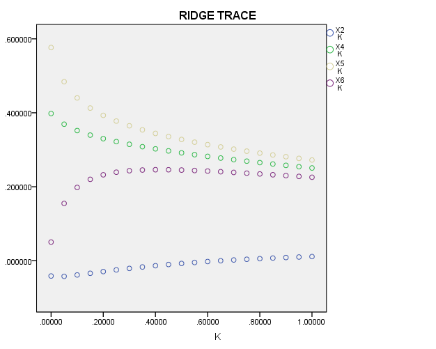
Figure 3: Ridge trace of \( {X_{2}} \) , \( {X_{4}} \) , \( {X_{5}} \) and \( {X_{6}} \) (Shandong).

Figure 3 indicates that when the ridge parameter \( k \) changes within \( (0.2,0.4) \) , the ridge traces of the other independent variables are basically stable. By \( {R^{2}} \) and equation significance comparison, it is found that when \( k=0.22 \) , the ridge regression model is optimal, and the parameters are as follows:

Table 10: Ridge regression coefficient table (Shandong).

This research aims to discuss the variables that have a significant impact on GDP. Table 10 indicates that at the test level of 0.05, the p-value of \( {X_{2}} \) is greater than 0.05, there is no evidence that \( {X_{2}} \) is significant to Shandong’s GDP. Therefore, ridge regression should be performed after removing variable \( {X_{2}} \) .

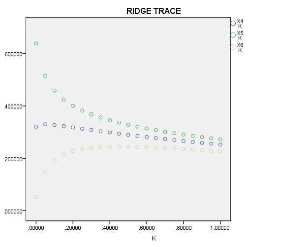
Figure 4: Ridge traces of \( {X_{3}} \) , \( {X_{4}} \) and \( {X_{6}} \) (Shandong).

4.2.4.2. Modified model

Figure 4 indicates that when the ridge parameter \( k \) changes within \( (0.2,0.4) \) , the ridge traces of the other independent variables are basically stable. By \( {R^{2}} \) and equation significance comparison, it is found that when \( k=0.2 \) , the ridge regression model is optimal, and the parameters are as follows:

Table 11: Revised ridge regression coefficient table (Shandong).

Table 12: Model summary table (Shandong).

The ridge regression equation can be obtained from Table 11 as follows:

\( Y=-16068.082+1.079{X_{3}}+1.506{X_{4}}+3.451{X_{6}} \) (5)

(5) indicates that when other conditions remain unchanged, residents' disposable income increases by 1 yuan, Shandong's GDP increases by an average of 1.079 billion yuan. When other conditions remain unchanged, each increase in industrial added value of 1 billion yuan will increase Shandong's GDP by 1.506 billion yuan on average. When other conditions remain unchanged, the added value of primary industry increases by 1 billion yuan, and Shandong's GDP increases by 3.451 billion yuan on average.

4.2.5. Model prediction effect analysis

Based on model (5), residents' disposable income, industrial added value and the added value of primary industry are taken as independent variables. The predicted GDP of Shandong from 2010 to 2022 is calculated and compared with the real value. The results show that the \( δ \) of the predicted and the real value in each year is all within 4%, and the mean and median of \( δ \) are about 1.5%, indicating that the predicted GDP is close to the real value, indicating that the model has a good degree of fitting. It has general applicability. The above data show that residents' disposable income, industrial added value and the added value of primary industry are three important factors for Shandong's GDP growth. The model fitting figure is as follows.

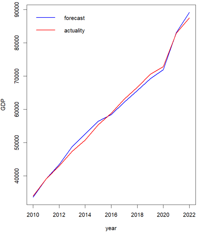
Figure 5: model fitting figure (Shandong).

5. Discussion

5.1. Similarities

Both Guangdong and Shandong regard residents’ disposable income and industrial added value as factors that significantly affect GDP. When residents' disposable income increases, their spending power and purchasing power will also increase, which further promotes domestic demand and drives economic growth. These two provinces both have a developed industrial base, and the manufacturing output value and industrial output value of the two provinces occupy an important position in the economy of the whole country. Therefore, industrial added value as a key indicator which has a significant influence on the economic performance of Guangdong and Shandong. If Guangdong and Shandong are used to represent the northern and southern provinces of China respectively, it can be seen that residents’ disposable income and industrial added value are important economic factors in both southern and northern provinces.

5.2. Differences

Guangdong regards the added value of real estate as the main factor that significantly affects GDP. According to the regression coefficient of model (3), among the three factors, the added value of real estate has the greatest impact on Guangdong's GDP. The real estate industry is one of the components of the tertiary industry. Not only the tertiary industry in Guangdong is the first of the three industries, but also the development potential of Guangdong has attracted a large number of population and investment. Therefore, the real estate industry is one of the important pillars of Guangdong's economy.

Shandong regards the added value of the primary industry as the main factor that significantly affects GDP. Shandong Province has vast farmland and abundant agricultural products resources, and the government attaches great importance to agricultural development. Through a series of policies and measures to support agriculture, Shandong has accelerated agricultural modernization, which is helpful to improve the added value of the primary industry, and then has a significant impact on GDP.

If Guangdong and Shandong are used to represent the northern and southern provinces of China respectively, it can be seen that the southern provinces have a good development prospect for the tertiary industry on account of geographical advantages and investment potential, while the northern provinces have a rapid development of the primary industry owing to resource advantages and policy support.

6. Conclusion

In conclusion, this paper intended to predict the GDP by demonstrating linear regression models, taking Guangdong Province and Shandong Province as examples. Guangdong and Shandong are the strongest economic provinces in southern and northern China respectively, this is also to observe economic characteristics of northern and southern China through these two representative provinces. This paper started with explaining the benefits of exploring important economic factors through linear models to China's economic development. Then the second part examined the works that have been done previously in the field. Last, final discussions were made of the comparisons with Guangdong’s GDP model and Shandong’s GDP model. With the foundation of existing research, this paper developed the prediction based on the ridge regression model, which makes the regression coefficient of the linear model more practical. In terms of practical application, the research conclusion contributed to China's North-South regional cooperation and the development of characteristic industries.

There are two major limitations in this study that could be addressed in future research. First, the study is limited to independent variables for residents' economic activities and industrial structure. More significant variables might not be included in the model. Second, the established regression models are based on historical data, which means that future temporal changes may lead to model inaccuracy. At the present state of knowledge, there are some important lessons for practice and research. Future studies can include more economic variables with local characteristics into the research scope, while time series analysis can be considered, which is conducive to observing the trend of economic indicators and better predicting the evolution of GDP.

References

[1]. Liu Wei. (2018). GDP and Development Outlook -- The Change of Development Outlook from the Understanding of GDP Since the Reform and Opening up. Economic Science, 02, 5-15.
[2]. Huang Xiaoyi. (2018). The Influencing Factors of Regional Gross Domestic Product Based on Multiple Linear Regression Analysis. Science Economy Society, 04, 76-78.
[3]. Wu Shiping, Zhang Jiaming & Zhu Haidong. (2018). Establishment of Guangdong Province’s GDP Model Based on Multiple Linear Regression. Journal of Foshan University (Natural Science Edition), 02, 27-30.
[4]. Yang Qing. (2020). The Influencing Factors of GDP in Hebei Province Based on Multiple Regression Model. Guangxi Quality Supervision Guide Periodical, 07, 210-211.
[5]. Zheng Wei, Zhang Ruishu & Guan Nanxing. (2019). Multiple Linear Regression Analysis of GDP Growth Driven by Three Industries: Based on 1998-2017 Data. Statistics and Management, 06, 9-12.
[6]. Jiang Bingye. (2019). Exploring Factors Affecting Real GDP Per Capital Based on Visualization and Multiple Linear Regression. Value Engineering, 29, 11-14.
[7]. Bai Yu. (2019). An Empirical Analysis of the Factors Influencing China's GDP Based on the Multiple Regression Analysis. Management & Technology of SME, 02, 55-57.
[8]. Guan Yongqian. (2021). Influencing Factors of GDP in Henan Province Based on Multiple Linear Regression. Rural Economy and Science-Technology, 05, 221-224.
[9]. Liang Haoan. (2021). Empirical study on influencing factors of GDP in Anhui Province -- Based on Multiple Regression Analysis. Times Finance, 24, 73-75.
[10]. Zhu Wanning. (2022). Analysis of Influencing Factors of Regional GDP in Anhui province Based on Multiple Linear Regression Model. Modern Business, 17, 90-94.
[11]. Wang Ning. (2018). The Influencing Factors of Economic Growth in Shandong Province Based on Multiple Linear Regression Model. Modern Business, 08, 68-70.
[12]. Li Yanfu. (2019). Study on Influencing Factors of Jiangsu GDP Based on Multiple Linear Regression Model. Special Zone Economy, 04, 84-88.
[13]. Xue Qian, Mou Fengyun & Tu Zhifeng. (2017). Application of Combination Forecast Method to Chongqing’s GDP Prediction. Journal of Chongqing Technology and Business University(Natural Science Edition), 01, 56-63.
[14]. Wang Hongchao & Wang Honglei. (2018). Forecasting of GDP Based on Exponential Smoothing and Regression Analysis. Economic Research Guide, 07, 1-6.
[15]. Liu Liu. (2017). GDP Forecasting of Gansu Province during the ‘13th Five-year Plan’ Period Based on Linear Regression. Journal of Huaihai Institute of Technology (Humanities and Social Sciences Edition), 03, 90-92.
[16]. A.E. Hoerl & R. W. Kennard. (1970). Ridge Regression: Biased Estimation for Nonorthogonal Problems. Technometrics, 1970, 12, 55-58.
Cite this article
Fang,Z. (2024). Application of Linear Regression in GDP Forecasting. Advances in Economics, Management and Political Sciences,72,92-104.
Data availability
The datasets used and/or analyzed during the current study will be available from the authors upon reasonable request.
Disclaimer/Publisher's Note
The statements, opinions and data contained in all publications are solely those of the individual author(s) and contributor(s) and not of EWA Publishing and/or the editor(s). EWA Publishing and/or the editor(s) disclaim responsibility for any injury to people or property resulting from any ideas, methods, instructions or products referred to in the content.
About volume
Volume title: Proceedings of the 2nd International Conference on Management Research and Economic Development
© 2024 by the author(s). Licensee EWA Publishing, Oxford, UK. This article is an open access article distributed under the terms and
conditions of the Creative Commons Attribution (CC BY) license. Authors who
publish this series agree to the following terms:
1. Authors retain copyright and grant the series right of first publication with the work simultaneously licensed under a Creative Commons
Attribution License that allows others to share the work with an acknowledgment of the work's authorship and initial publication in this
series.
2. Authors are able to enter into separate, additional contractual arrangements for the non-exclusive distribution of the series's published
version of the work (e.g., post it to an institutional repository or publish it in a book), with an acknowledgment of its initial
publication in this series.
3. Authors are permitted and encouraged to post their work online (e.g., in institutional repositories or on their website) prior to and
during the submission process, as it can lead to productive exchanges, as well as earlier and greater citation of published work (See
Open access policy for details).