


1. Introduction
In the era of the pandemic, consumers’ daily needs and consumption habits tend to be “pandemic-oriented,” and supermarkets often face absurd situations of being “emptied out.” Although the shadow of the pandemic is gradually receding, the challenges of inventory management persist for numerous managers, especially in the case of fresh produce. Given the difficulty in preservation and the short shelf life of fresh products, dynamic replenishment and pricing decisions are necessary on a daily basis, posing significant challenges for supermarkets. This paper, based on the provided sales data of relevant vegetable products, formulates model assumptions and provides corresponding solutions, offering simple conceptual guidance for real-world supermarket management.
Firstly, let’s outline the existing issues:
Issue One: It is necessary to clarify the distribution patterns and interrelationships of sales volumes among different individual items and categories of vegetable products. By doing so, we can identify the sales relationships among individual items and categories. Simultaneously, based on the sales distribution curves, we can observe distinctive fluctuation patterns in certain individual items and categories.
Issue Two: Building on the identified sales distribution patterns for each category, we aim to forecast the daily sales data for the upcoming week. Utilizing the cost-plus pricing method [Selling Price = Wholesale Price * (1 + Cost Markup Rate)], assuming the independent variable x represents the cost markup rate, we can derive the relationship between the total sales volume y and the independent variable x. Combining the loss rate for each category allows us to express the replenishment quantity in terms of the sales volume y. By considering profit as revenue minus cost, we can formulate a comprehensive profit expression in terms of x. Consequently, we can determine the value of x that maximizes profit, leading to optimal daily replenishment quantities and pricing strategies that maximize supermarket returns.
Issue Three: Focusing on individual items within the identified categories, we further operationalize the approach. The objectives include controlling the total number of individual items between 27-33, ensuring each item’s order quantity is not less than 2.5kg, considering the available types of sellable items from the previous week, and maximizing supermarket returns. In other words, optimal decisions must be made while satisfying the first three requirements, achieving the best possible strategy within the constraints outlined.
2. Literature Review
Supermarkets manage a diverse range of products in large quantities, and in order to adapt to market diversity and meet the shopping needs of customers, operators must enhance their management skills [1]. This is especially true for perishable goods, which pose a severe challenge to the management of supermarkets. The task is to balance the diverse consumption needs of shoppers while maximizing the supermarket’s profitability. Liu Liping et al. (2001) analyzed beverage sales in supermarkets using a regression analysis model [2]. Huang Xiaomei (2013) utilized simple linear regression analysis to establish a sales prediction model for beverages. Additionally, she employed Matlab software to analyze the correlation between daily beverage sales and the daily maximum temperature in supermarkets [3]. Kuo (1998) focused on a specific milk product in a convenience store in Taiwan, constructing a fuzzy neural network model based on the historical sales of the product over the past year. The study identified four categories containing a total of 17 influencing factors affecting the sales of this product through a questionnaire survey [4]. Doganis et al. (2006) used nonlinear time series to establish a mid-term sales forecasting model for fresh milk products in a food retail enterprise [5].
3. Model Assumptions and Symbolic Representation
3.1. Model Assumptions
3.1.1. Assumption 1: In the provided data, only the loss rate and wholesale price impact the cost of goods. This paper considers only the influence of the loss rate and wholesale price on supermarket returns, neglecting other factors such as labor costs that may affect profits.
3.1.2. Assumption 2: When using time series models for sales volume fitting, other factors influencing sales volume, such as weather, market competition, and buyer purchasing behavior, are not considered.
3.1.3. Assumption 3: In calculating the daily average selling price for each category, this paper uses the mean selling price of each category to represent the daily selling price of the category. The weighting of individual items within the category is not considered. For discounted vegetables, they are treated the same as regular vegetables in calculating the mean, without any additional adjustments.
3.2. Symbolic Representation
Table 1. Symbolic representation
Symbolic Hypothesis | Symbol Description |
| Observations of objects on features in the observation matrix |
| Standardized Euclidean distance, sample<i mtid=‘144’>hello</i> and samples <i mtid=‘146’>hello</i> the similarity coefficient between them |
| Profit from selling vegetables after deducting losses |
| Cost markup rate |
| sales volume |


4. Model Establishment and Solution
4.1. Analysis and Modeling of Problem One
4.1.1. Data Preprocessing: Initially, the data underwent cleaning using Stata to merge and integrate the data from attachments one and two. Upon examination, five individual items, namely local spinach, cordyceps flowers (box) (1), Wuhu green peppers (portion), lotus roots, and Wuhu green peppers (2), were found to lack both purchase and sales records. These items were directly excluded. Subsequently, processing was performed on the merged dataset comprising over 870,000 records to obtain daily sales volumes for each individual item. A box plot was then employed to eliminate extreme data points beyond the box boundaries. Finally, the remaining data underwent cluster analysis.
4.1.2. Cluster Analysis Model: Cluster analysis reveals the inherent structure and patterns within data through multivariate statistical values, categorizing samples based on similarity while separating dissimilar samples. This process aids in simplifying data processing complexity and can be viewed as a form of dimensionality reduction. To address the relationship between different individual items and sales volumes, cluster analysis was employed after filtering out invalid data. A total of 1,086 samples remained after the data cleansing process. These processed data were input into SPSS for cluster analysis, yielding the following results:
For a given set of m objects to be classified, denoted as \( {X_{1}},{X_{2}},⋯,{X_{m}} \) , described by n features, the observation matrix of m objects on n features is represented as:
\( X=(\begin{matrix}\begin{matrix}{x_{11}} & {x_{12}} \\ {x_{21}} & {x_{22}} \\ \end{matrix} & ⋯ & \begin{matrix}{x_{1n}} \\ {x_{2n}} \\ \end{matrix} \\ ⋮ & ⋱ & ⋮ \\ \begin{matrix}{x_{m1}} & {x_{m2}} \\ \end{matrix} & ⋯ & {x_{mn}} \\ \end{matrix}) \)
The process of hierarchical cluster analysis is outlined as follows:
The hierarchical cluster analysis method is widely applied, with the basic idea being to initially treat each sample as an independent class. Subsequently, a similarity measure is employed to evaluate the degree of similarity among all samples. The most similar samples are then aggregated into a small class. This process is iteratively repeated, with the current most similar sample or class being aggregated into a category until all samples are finally aggregated into a complete category. To investigate the relationship between sales volumes of different individual items, hierarchical cluster analysis was employed.
For distance measurement, we adopted standardized Euclidean distance:
\( d({x_{i}},{x_{j}})={[\frac{1}{m}\sum _{k=1}^{p}{({x_{ik}}-{x_{jk}})^{2}}]^{\frac{1}{2}}} \) (i,j=1,2, \( ⋯ \) ,n)
Here, \( d({x_{i}},{x_{j}}) \) represents the similarity coefficient between samples \( {x_{i}} \) and \( {x_{j}} \) ; m denotes the number of variables; n denotes the number of samples; \( {x_{ik}} \) represents the value of the k-th variable of sample i, and \( {x_{jk}} \) represents the value of the k-th variable of sample j. The processed data were then input into SPSS for cluster analysis, and the results were obtained. To optimize the model and determine the appropriate k value, the elbow method was employed, estimating the optimal clustering quantity k through MATLAB’s plot of the clustering coefficient line graph for individual items and sales volume. From this graph, it is evident that the descending speed is slow at the inflection point of 2. Consequently, the k value was set to 4, dividing individual items into four clusters using the k-means algorithm.
Through cluster analysis, more than two hundred individual items were categorized into four clusters. The first cluster comprises Wuhu green peppers (1), the second cluster includes Net Lotus Roots (1), the third cluster consists of Chinese cabbage, and the fourth cluster encompasses other vegetables. The cluster dendrogram reveals strong correlations between Yunnan lettuce, purple eggplant (2), and broccoli, as well as positive correlations among Chinese cabbage, amaranth, and bell peppers. Spinach (portion), Yunnan oilseed rape (portion), and small bell peppers (portion) also exhibit strong correlations. All these relationships are positive, suggesting that the supermarket can bundle and sell these vegetables together to promote mutual sales growth, thereby achieving the ultimate goal of pursuing higher economic benefits. Similarly, we present a spectral graph of category versus total sales volume, as shown in Figure 1, and provide a distortion degree curve:
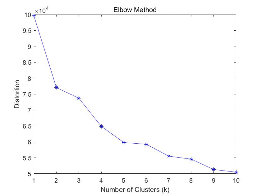
Figure 1. Distortion degree curve
It can be observed that when k=2, it is the obvious inflection point, allowing the categorization into two major clusters: leafy vegetables and others. Considering the mutual relationships among these six categories, it is evident that leafy vegetables, solanaceous vegetables, and aquatic tuber vegetables complement each other. Chili peppers and edible fungi also exhibit a strong correlation, while leafy vegetables have a negative correlation with aquatic tuber vegetables and chili peppers. This implies that leafy vegetables are substitutes for aquatic tuber vegetables and chili peppers. Other categories show positive correlations, indicating mutual promotion among them, serving as complementary products. Notably, there is a strong correlation between aquatic tuber vegetables and edible fungi, as well as between chili peppers and edible fungi, compared to other categories.
4.2. Model Analysis and Formulation for Problem Two
4.2.1. Solution and Results for Model Two. To determine the optimal daily replenishment quantities and pricing strategies for various vegetable categories over the next week, aiming to maximize the supermarket’s returns, we utilized the establishment of an optimization model to describe the relationship between total profit, individual product sales volume, and purchase cost.
The optimization model for the problem is as follows:
1. Decision Variables:
\( {x_{ij}},(j=1,2,⋯,6) \)
Representing leafy vegetables, cruciferous vegetables, chili peppers, solanaceous vegetables, edible fungi, and aquatic tuber vegetables, respectively.
2. Objective Function:
\( Z total=\sum _{i=1}^{7}{w_{i1}}+{w_{i2}}+{w_{i3}}+{w_{i4}}+{w_{i5}}+{w_{i6}} \)
3. Constraints:
\( maxW total=\sum _{i=1}^{7}\sum _{j=1}^{6}{W_{ij}} \)
s.t. \( \begin{cases} \begin{array}{c} \begin{matrix}{y_{ij}}={a_{j1}}+{a_{j2}}{x_{ij}} \\ \begin{matrix}{y_{ij}}=(1+{w_{ij}}){c_{ij}} \\ \begin{matrix}{W_{ij}}={w_{ij}}×{x_{ij}} \\ \begin{matrix}{x_{ij}},{y_{ij,{W_{ij}} ≥0}} \\ \end{matrix} \\ \end{matrix} \\ \end{matrix} \\ \end{matrix} \\ {W_{ij}}∈{R^{+}} \end{array} \end{cases} \) Where, i=(1,2, \( ⋯,7 \) ),j=(1,2, \( ⋯ \) ,6)
4.3. Analysis and Modeling for Problem Three
4.3.1. Formulation of Model Three. In order to assist the supermarket in formulating a more scientific replenishment plan for individual items under a limited number of saleable items, aiming to maximize the supermarket’s profit, we typically select items with higher net profits.
\( [Here, the net profit of an individual item is calculated as W=(averagesellingprice-averagewholesaleprice)×totalsalesquantity×(1-lossrate)] \)
However, in reality, the net profit of individual items is easily influenced by occasional large purchases from certain customers. Therefore, using the net profit of individual items as the sole indicator for formulating replenishment plans is not scientific. Instead, we should also consider the purchase frequency of a particular item.
First, we perform preliminary data processing, filtering out 49 saleable items from June 24th to June 30th. Then, we construct a standardized matrix consisting of 49 objects and 2 evaluation indicators.
\( Z=[\begin{matrix}{z_{11}} & {z_{12}} \\ ⋮ & ⋮ \\ {z_{49 1}} & {z_{49 2}} \\ \end{matrix}] \)
Define the maximum values \( {Z^{+}}=(Z_{1}^{+},Z_{2}^{+})=(max\lbrace {z_{11}},{z_{21}},⋯,{z_{49 1}}\rbrace ,max\lbrace {z_{12}},{z_{22}},⋯,{z_{49 2}}\rbrace ) \)
Define the minimum values \( {Z^{-}}=(Z_{1}^{-},Z_{2}^{-})=(min\lbrace {z_{11}},{z_{21}},⋯,{z_{49 1}}\rbrace ,min\lbrace {z_{12}},{z_{22}},⋯,{z_{49 2}}\rbrace ) \)
Define the distance from the i-th (i = 1,2, ...,49) evaluation object to the maximum value \( D_{i}^{+}=\sqrt[]{\sum _{j=1}^{2}{{w_{1}}(Z_{j}^{+}-{z_{ij}})^{2}}} \)
Define the distance from the i-th (i = 1,2, ...,49) evaluation object to the minimum value \( D_{i}^{\_}=\sqrt[]{\sum _{j=1}^{2}{{w_{2}}(Z_{j}^{\_}-{z_{ij}})^{2}}} \)
Then, it is easy to calculate the non-normalized score for the i-th (i = 1,2, ...,49) evaluation object: \( {S_{i}}=\frac{D_{i}^{-}}{D_{i}^{+}+D_{i}^{-}} \) , where \( 0≤{S_{i}}≤1 \) .
Next, based on the original data, we use the TOPSIS method to calculate the comprehensive scores. Initially, we utilize expert estimation to assign weights to the two indicators, giving the weights as W = (0.3,0.7).
The final normalized matrix is:
\( Z=[ \begin{array}{c} \begin{matrix}0.0074 & 0.0340 \\ 0.0556 & 0 \\ \end{matrix} \\ \begin{matrix}⋮ & ⋮ \\ 0.6444 & 0.4999 \\ \end{matrix} \\ \begin{matrix}⋮ & ⋮ \\ 0.7889 & 0.2491 \\ \end{matrix} \\ \begin{matrix}0.5148 & 0.3411 \\ \end{matrix} \end{array} ] \)
According to the formula \( K=0.3×{z_{i1}}+0.7×{z_{i2}} (where i=1,2,⋯,49) \) , we calculate the comprehensive scores. Removing items whose order quantity does not meet the minimum display quantity of 2.5 kilograms, we finally select 30 items:
Xiaomi Pepper (portion), Broccoli, Yunnan Lettuce (portion), Wuhu Green Pepper (1), Xixia Flower Mushroom (1), Yunnan Oil Wheat Vegetable (portion), Bamboo Leaf Vegetable, Clean Lotus Root (1), Purple Eggplant (2), Screw Pepper, Honghu Lotus Root Strip, Baby Cabbage, Double-Spore Mushroom (box), Long Eggplant, Wood Ear Vegetable, Screw Pepper (portion), Amaranth, Milk White Cabbage, Small Wrinkled Skin (portion), Enoki Mushroom (box), Small Chinese Cabbage (1), Ginger Garlic Xiaomi Pepper Combo (small portion), Red Pepper (2), Shanghai Green, Sweet Potato Tip, Spinach (portion), Seafood Mushroom (pack), Gao Gua (1), Seven-Color Pepper (2), Zhijiang Green Stem Loose Flower.
Then, we use time series models to predict the sales volume of these 30 items on July 1st. According to the formula, Dailyreplenishmentquantity= Salesvolume /(1- lossrate), we obtain the replenishment quantities for these 30 items.
We convert the problem of maximizing the revenue from items sold on July 1st into a 0-1 integer programming problem. Introducing the variable m, where m=0 indicates that the item was not sold, and m=1 indicates that the item was sold. Let Q represent the total profit, ai represent the pricing, ci represent the profit rate, and yi represent the cost price.
\( ai=(1+ci)*yi \)
\( Q=ci*yi \)
\( max Q=\sum _{i=1}^{30}miciyi \)
\( \begin{cases} \begin{array}{c} ai=(1+ci)*yi \\ mi=0or1 \\ ci,yi≥0 \\ i=1……30 \end{array} \end{cases} \)
4.3.2. Solution of Model Three and Results
Table 2. Category sales strategy
Single product name | Total daily replenishment amount (kg) | Pricing strategy (%) |
Gaogua | 18.37 | 62.54 |
Sweet potato tip | 16.53 | 47.82 |
Auricularia auricula | 6.82 | 90.13 |
Clean lotus root | 34.56 | 32,79 |
broccoli | 28.65 | 58.36 |
Amaranth | 7.86 | 88.34 |
Bamboo leafed vegetable | 15.77 | 48.96 |
Finally, the replenishment quantities and pricing strategies for each category have been determined, providing a reference for the procurement and pricing of fresh vegetables in the supermarket.
5. Conclusion
This paper discusses the complex issues of procurement and pricing of fresh vegetables in supermarkets. Utilizing methods such as hierarchical clustering analysis, Topsis evaluation, and optimization models, the paper constructs data models and establishes multiple models to address the formulation of replenishment and pricing decisions from various perspectives and levels. The research reveals the following key findings: Firstly, the paper categorizes vegetable products into four clusters and explores the complementary and substitute relationships within them. It identifies reasonable sales combinations among different types of products, fostering mutual promotion of sales and enabling supermarkets to achieve higher economic benefits. Secondly, the paper develops a mathematical model describing the relationship between total profit, individual product sales, and pricing. This model provides valuable recommendations for supermarkets’ replenishment quantities and pricing decisions, ensuring practical support for the implementation of pricing and replenishment plans. Thirdly, the paper establishes a model for maximizing profits while keeping replenishment quantities constant. This model aids supermarkets in formulating scientifically sound replenishment plans for a limited number of sellable products. By judiciously applying the innovative mathematical models proposed in this paper, supermarkets can obtain reliable market analyses and make corresponding replenishment and pricing decisions.
References
[1]. Cui, K. F. (Year not provided). Design and Implementation of Supermarket Commodity Management System.
[2]. Liu, L. P., Ding, J. J., & Qin, T. (2001). Application of Regression Analysis in Beverage Sales Forecasting. Statistics and Forecasting, 2001(06).
[3]. Huang, X. M. (2013). Application of Simple Linear Regression Analysis in Supermarket Product Sales. Science and Technology Information, 2013(11).
[4]. R.J. Kuo; K.C. Xue. A decision support system for sales forecasting through fuzzy neural networks with asymmetric fuzzy weights. [J]. Decision Support Systems.1998(2)
[5]. Philip Doganis; Alex Alexandridis; Panagiotis Patrinos; Haralambos Sarimveis. Time series sales forecasting for short shelf-life food products based on artificial neural networks and evolutionary computing. [J]. Journal of Food Engineering.2005(2)
Cite this article
Chen,Y.;Zheng,Z.;Wang,X.;Meng,Z.;Li,J. (2024). Automatic pricing and replenishment decision-making for vegetable products based on optimization models. Theoretical and Natural Science,34,291-297.
Data availability
The datasets used and/or analyzed during the current study will be available from the authors upon reasonable request.
Disclaimer/Publisher's Note
The statements, opinions and data contained in all publications are solely those of the individual author(s) and contributor(s) and not of EWA Publishing and/or the editor(s). EWA Publishing and/or the editor(s) disclaim responsibility for any injury to people or property resulting from any ideas, methods, instructions or products referred to in the content.
About volume
Volume title: Proceedings of the 3rd International Conference on Computing Innovation and Applied Physics
© 2024 by the author(s). Licensee EWA Publishing, Oxford, UK. This article is an open access article distributed under the terms and
conditions of the Creative Commons Attribution (CC BY) license. Authors who
publish this series agree to the following terms:
1. Authors retain copyright and grant the series right of first publication with the work simultaneously licensed under a Creative Commons
Attribution License that allows others to share the work with an acknowledgment of the work's authorship and initial publication in this
series.
2. Authors are able to enter into separate, additional contractual arrangements for the non-exclusive distribution of the series's published
version of the work (e.g., post it to an institutional repository or publish it in a book), with an acknowledgment of its initial
publication in this series.
3. Authors are permitted and encouraged to post their work online (e.g., in institutional repositories or on their website) prior to and
during the submission process, as it can lead to productive exchanges, as well as earlier and greater citation of published work (See
Open access policy for details).
References
[1]. Cui, K. F. (Year not provided). Design and Implementation of Supermarket Commodity Management System.
[2]. Liu, L. P., Ding, J. J., & Qin, T. (2001). Application of Regression Analysis in Beverage Sales Forecasting. Statistics and Forecasting, 2001(06).
[3]. Huang, X. M. (2013). Application of Simple Linear Regression Analysis in Supermarket Product Sales. Science and Technology Information, 2013(11).
[4]. R.J. Kuo; K.C. Xue. A decision support system for sales forecasting through fuzzy neural networks with asymmetric fuzzy weights. [J]. Decision Support Systems.1998(2)
[5]. Philip Doganis; Alex Alexandridis; Panagiotis Patrinos; Haralambos Sarimveis. Time series sales forecasting for short shelf-life food products based on artificial neural networks and evolutionary computing. [J]. Journal of Food Engineering.2005(2)