1. Introduction

The Reuleaux triangle is an astonishing figure which belongs to the big family of bodies of constant width and can be constructed by constructing three identical circles together. The ‘constant width’ means that if we put the figure between two parallel straight lines while the two lines are both tangent to the curve, no matter how the figure rotates or moves, the two lines are always tangent to it. As a result, the Reuleaux triangle is a mysterious figure and it has been studied by scientists after it was originally discovered by the German mathematician and mechanist Lelo during the 19th century[1]. The discovery of Reuleaux triangle brought many inspirations for scientists and the expression ‘constant width figure’ to the Maths scene. Moreover, this geometric figure has even been applied in several practical regions such as the construction of cars and some transmission devices which reflects the great potential of this amazing figure.

This paper not only sets out to analyse and demonstrate some of the Reuleaux triangle’s basic theoretical features and a few ideas expanded from its features but also involves some considerable approaches to putting the Reuleaux triangle into practice and the corresponding proofs which prove the feasibility and the practicability of the approaches. To be more specific, the content of this paper would be divided into the theoretical part and the practical part. The theoretical part would contain two different types of methods to prove that the Reuleaux triangle is a constant width figure, it would also discuss the question of what if the idea of the Reuleaux triangle is expanded into more than 3 arc-sided figures and so whether some of the original features would change. Moreover, the approaches of drawing constant width figures would be included as well, this idea would also be developed to discover the possible rules inside the problem. By contrast the idea of finding an exact way to stable the car when traveling using Reuleaux triangle-shaped wheels would rather be involved in the practical part. Furthermore, the investigation of using the Reuleaux triangle-shaped drills to drill square holes would be in the practical part too. In addition, the practical part would include the demonstration to find the equation of the locus of the centre point of the triangle and whether the integrity of the square is not related to its centre point’s movement or with the triangle’s size which is related to the topic.

Overall, the final aim of the study is to work out the practical uses of the Reuleaux triangle based on its theoretical features so as to bring some new ideas in areas such as transportation, and the demonstrations themselves may be helpful for people who would like to study further into this topic.

2. Methodology

The paper would mainly involve analytic geometry, differentiation in the proofs and demonstrations, and graphs would be used as an auxiliary tool to help the paper to be more understandable.

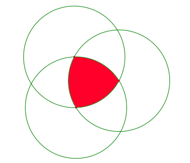Figure 1. The Reuleaux triangle(painted red) constructed by three identical circles.

In order to prove that the Reuleaux triangle(see figure 1) is a constant width curve, this paper would first put the triangle in a coordinate system and then choose two points on the sides of the triangle. Then this paper would express the coordinate of the two points by an independent variable and use the formula of the distance between 2 points to demonstrate that the maximum value of the distance is always the same. As a result, the proposition of the Reuleaux triangle having a constant width can be proved correct. The formula for the distance between two points in a coordinate system goes: \( \)

\( d=\sqrt[]{{({x_{1}}-{x_{2}})^{2}}+{({y_{1}}-{y_{2}})^{2}}} \) (1)

while \( ({x_{1}},{y_{1}}) \) and \( ({x_{2}},{y_{2}} \) ) are the coordinates of the two points.

In addition, expertise about the differentiation would also be applied so as to find out the features of functions that We use in the proof. Moreover, this part mainly consists of the first and second derivatives. Apart from that the first derivative would be applied as it can show the monotonicity characteristics of the original function: Assume that the original function is \( f(x) \) then if \( f \prime (x) \) is positive, the original function monotonically increases in its domain, and if \( f \prime (x) \) is negative, the original function monotonically declines in its domain but when \( f \prime (x) \) equals to zero, which means the original function reaches an extreme value. In addition, the second derivative would also be used in order to learn whether the extreme point is the maximum point or the minimum point: Firstly, work out the value of x when \( f \prime (x) \) reaches zero. Then substitute the value into \( f \prime \prime (x) \) which is the second derivative of the original function, if the result is positive the point is the minimum point and if the result is negative the point is the maximum point of the graph. Overall, the information above would be used to work out the situation when the distance between the two points reaches a maximum value. To find the equation of the locus of the centre point of the Reuleaux triangle when it rotates on a straight line, the paper would not only use the knowledge of geometry and trigonometry but also the induction formulas. It is known that the median, perpendicular, and angular bisector of a triangle would always intersect at a point. Thus, it can be demonstrated that for a regular triangle, the coordinate of its centre point is just the average of the coordinates of the triangle’s three vertexes. Moreover, the induction formulas are mainly used to simplify the result as it would contain several compound trigonometric functions and the formulas are (a&b are both values of the unknown degrees):

\( sin{(a+b)=sin{acos{b+sin{bcos{a}}}}} \)

\( sin{(a-b)=sin{acos{b-sin{bcos{a}}}}} \)

\( cos{(a+b)=cos{a}cos{b}-sin{a}sin{b}} \)

\( cos{(a-b)=cos{a}cos{b}+sin{a}sin{b}} \) (2)

As for the approach of drawing more constant width curves, the method would be analyzed rigorously and the possible rules inside would be demonstrated. However, as the problem is hard to be solved by the mathematical induction, and the expertise is restricted, the paper would rather use theoretical reasoning and graphs to demonstrate the rule and the exact approach of drawing any constant width curve with sides of even number.

The paper would also use properties of Polar form and Euler form of complex numbers, which goes: \( {e^{iθ}}=cosθ+isinθ \) , to calculate the equation of locus when it rotates to form a square.

3. The two approaches to proving that the Reuleaux triangle has a constant width

Proof 1:

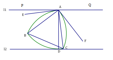Figure 2. The Reuleaux triangle between two parallel straight lines.

In order to prove that the Reuleaux triangle has constant width, we need to find a variate that can be regarded to be related to the length between two points on the curve. Then if we are able to prove that the alter of the variate would not affect the maximum distance between the two points, the constant width of the Reuleaux triangle can be successfully proved.

As it is shown in Figure 2, a Reuleaux triangle is located between two parallel straight lines \( {l_{1}} \) and \( {l_{2}} \) , and the two lines are both tangent to the triangle at point A and point D respectively. Then we assume that ∠CAD equals to α and ∠BAD equals to β and we define that they are both strictly greater than 0 as this paper is only considering the situation in which one tangent point is point A and the other point locates on the arc BDC. We construct the line AE and AF which are both tangent to the curve are perpendicular to AC and AB respectively, thus it can be found that the arc AB and AC are always below line AE and AF respectively. What’s more, it is not hard to find out that ∠EAP equals to α and ∠FAQ equals to β due to the complementary of the angles on the graph. As it has been defined, α and β are both positive, which means no matter how we rotate the triangle, one of the lines AE and AF is always approaching line \( {l_{1}} \) but it can never reach it therefore point E and F are always both below the line \( {l_{1}} \) . Thus it can be demonstrated that point A is always the highest point under this situation which means that the length of AD is always the longest when \( {l_{2}} \) is tangent to the triangle on the arc BC. Hence it can be concluded that the curve is constant width and the length of AD, also the length of the radius of the circles used to construct the Reuleaux triangle is the length of the constant width.

However, although the former approach can demonstrate that the Reuleaux triangle is a constant width figure in an abstract and may be much more understandable, the second one is more rigorous and precise.

Proof 2:

To prove that the Reuleaux triangle has a constant width, we can choose two points on the curve and work out the distance between them[2]. In this part we construct a Reuleaux triangle in the coordinate system and let the length of the side of the inner triangle be 1 which means the radius of the circles used to construct the Reuleaux triangle is 1. As the graph shows, get two points on each side of the arc and mark them A and B. To prove that the Reuleaux triangle has constant width, we only need to prove that the distance between A and B has a maximum value while they are able to move freely on the arcs they are positioned on.

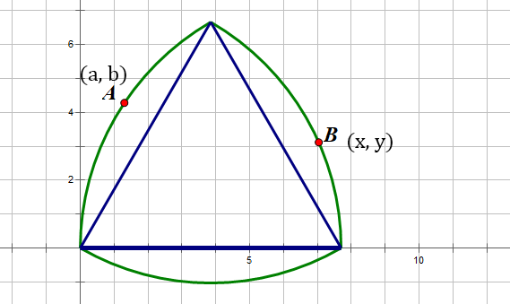Figure 3. The Reuleaux triangle constructed in the coordinate system with points A and B on its arcs.

However, studying two free-moving points at the same time is really complex and hard, thus we would like to fix point B and move point A on the arc. Let’s assume that the coordinates of A and B are \( (x, y) \) and \( (a, b) \) (as shown in Figure 3) respectively and the range of a would be \( [\frac{1}{2}, 1] \) and the range of b and y both are \( [0, \frac{\sqrt[]{3}}{2}] \) . as the arc point A is on is a part of the circle whose equation goes: \( {(x-1)^{2}}+{y^{2}} =1 \) and the arc point A is located on is belonged to the left part of the original circle, the coordinate of point A can also be expressed as \( (-\sqrt[]{1-{y^{2}}}+1, y) \) . Thus the coordinate of point B can be expressed as \( (a, \sqrt[]{1-{a^{2}}}) \) with the same reason as point A, but we shall use this later. Then according to the formula of the distance between two points mentioned in the methodology part, we can work out the distance between A and B:

\( Distance=\sqrt[]{{(-\sqrt[]{1-{y^{2}}}+1-a)^{2}}+{(y-b)^{2}}} \)

\( =\sqrt[]{2+2(a-1)\sqrt[]{1-{y^{2}}}-2a+{a^{2}}-2by+{b^{2}}} \)

\( =\sqrt[]{2(1-a)(1-\sqrt[]{1-{y^{2}}})+{a^{2}}-2yb+{b^{2}}} \) (3)

As the radical sign would exert an influence on the later differentiation and calculation, we assume that:

\( g(y)=2(1-a)(1-\sqrt[]{1-{y^{2}}})+{a^{2}}-2yb+{b^{2}} \) (4)

Now we differentiate the function \( g(y) \) to study its monotonicity characteristics and its extreme values:

\( {g \prime (y)=2(1-a)·y(1-{y^{2}})^{-\frac{1}{2}}}-2b \) (5)

According to the range of a, b the \( 2(1-a) \) and \( 2b \) are always positive, then we shall study about the \( {y(1-{y^{2}})^{-\frac{1}{2}}} \) and we assume it p(y):

\( {p(y)=y(1-{y^{2}})^{-\frac{1}{2}}} \)

\( {p \prime (y)={(1-y^{2}})^{-\frac{1}{2}}}+y{(1+{y^{2}})^{-\frac{3}{2}}} \) (6)

Because the range of y is \( [0, \frac{\sqrt[]{3}}{2}] \) , the range of \( {y^{2}} \) would be \( [0, \frac{3}{4}] \) . Thus it is easy to discover that the value of \( p \prime (y) \) is always positive, which means the original function p(y) is a monotonic increasing function on the domain \( [0, \frac{\sqrt[]{3}}{2}] \) . When y equals to \( \frac{\sqrt[]{3}}{2} \) , we assume the function \( g \prime (y) \) be f(a):

\( {f(a)=\sqrt[]{3}(1-a)-(1-{a^{2}})^{\frac{1}{2}}} \) (7)

We firstly work out the value of a when f(a) equals to zero:

\( {\sqrt[]{3}(1-a)-(1-{a^{2}})^{\frac{1}{2}}}=0 \)

\( a=\frac{1}{2} or a=1 \) (8)

Then we differentiate f(a):

\( f \prime (a)=a{(1-{a^{2}})^{-\frac{1}{2}}}-\sqrt[]{3} \) (9）

We work out the value of a while f’(a) equals to zero so as to find out the extreme point of the function f(a):

\( a{(1-{a^{2}})^{-\frac{1}{2}}}-\sqrt[]{3}=0 \)

\( a=\frac{\sqrt[]{3}}{2} \)

\( f(\frac{\sqrt[]{3}}{2})=\sqrt[]{3}-2 \) (10)

Then we use the second derivative to work out the characteristics of this extreme point:

\( f \prime \prime (a)={{(1-a^{2}})^{-\frac{1}{2}}}+y{(1+{a^{2}})^{-\frac{3}{2}}} \) (11)

As the value of f’’(a) is always positive in its domain, the point \( (\frac{\sqrt[]{3}}{2}, \sqrt[]{3}-2 \) ) is the minimum point of the original function. Also due to \( \sqrt[]{3}-2 \lt 0 \) , the value of f(a) is negative in the domain \( [\frac{1}{2}, 1] \) therefore the value of g’(y) is always negative, which means the function g(y) is a monotonic decreasing function in its domain \( [0, \frac{\sqrt[]{3}}{2}] \) .

Despite the value of a and b, the distance between A and B would reach a maximum value when y declines to the value of zero, which means point A is coincident with the original point, also one of the vertexes of the Reuleaux triangle. Hence there is always a maximum value of the distance between any two points on a Reuleaux triangle so that the Reuleaux triangle is a constant width curve.

4. The equation of locus when the Reuleaux triangle is rotating inside a square

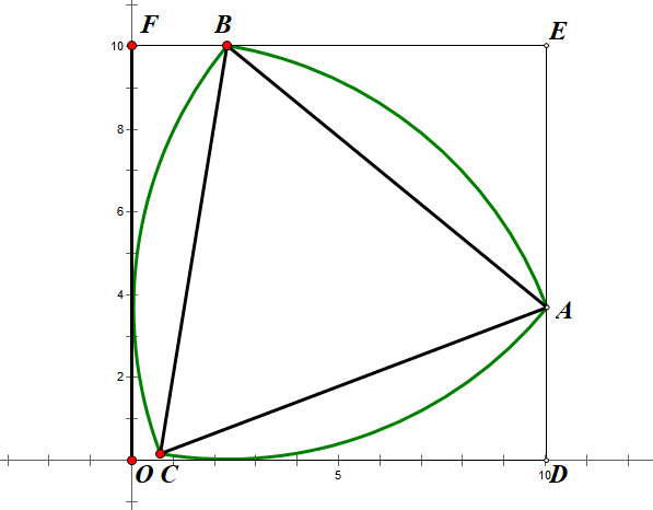
Many drills are Reuleaux triangle-shaped as when they rotate in a certain trail, a square hole would form so that it has been used in the area related to this. However, if we observe carefully we can discover that the centre point Reuleaux triangle is moving in a certain trail as it rotates and the four corners of the square are always arc-shaped. As a result, this paper would use the mathematical approaches to work out the equation of locus of the centre point and show the graph of it.

We first construct a complex plane and put a square and a Reuleaux triangle inside it, as Figure 4 shows.

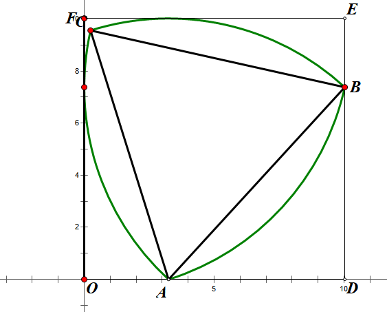Figure 4. A Reuleaux triangle inside a square.

It can be observed that among the triangle’s three vertexes, two of them are always on the sides of the square and the other vertex is always inside the square. Thus we can divide one complete period into four situations, and the situation shown in the Figure 4 is the first one. In order to express the coordinate of the center locus using parametric functions, we can firstly work out the coordinates of the three vertexes of the triangle.

Let’s assume that the side length of the square is 1 and the length of AD is equal to t, thus the coordinates of points A and B would be \( (1-t, 0) \) and \( (1, \sqrt[]{1-{t^{2}}}) \) respectively. Then we may express the vector AB \( (t, \sqrt[]{1-{t^{2}}}) \) , and we can then work out the expression of vector AC as it can just be formed by rotating AB sixty degrees around point A. Due to the relationship between Polar form and Euler form of complex number, which goes: \( {e^{iθ}}=cosθ+isinθ \) , and the fact that the triangle is constructed in a complex plane, we can express vector AC in the complex form:

\( vector AC=vector AB ×{e^{\frac{π}{3}i}} \)

\( =(t+i\sqrt[]{1-{t^{2}}})×{e^{\frac{π}{3}i}} \)

\( =(t+i\sqrt[]{1-{t^{2}}})×（cos\frac{π}{3}+isin\frac{π}{3}） \)

\( =(\frac{1}{2}t-\frac{\sqrt[]{3}}{2}\sqrt[]{1-{t^{2}}})+(\frac{\sqrt[]{3}}{2}t+\frac{1}{2}\sqrt[]{1-{t^{2}}})i \)

\( =(\frac{1}{2}t-\frac{\sqrt[]{3}}{2}\sqrt[]{1-{t^{2}}}, \frac{\sqrt[]{3}}{2}t+\frac{1}{2}\sqrt[]{1-{t^{2}}}) \) (12)

Thus we can work out the coordinate of the center point of the triangle by calculating the average value of the three vertexes’ coordinates. The result would be:

\( (1-\frac{1}{2}t-\frac{\sqrt[]{3}}{6}\sqrt[]{1-{t^{2}}}, \frac{\sqrt[]{3}}{6}t+\frac{1}{2}\sqrt[]{1-{t^{2}}}) \) (13)

In which the domain of t would be \( [\frac{1}{2}, \frac{\sqrt[]{3}}{2}] \) .

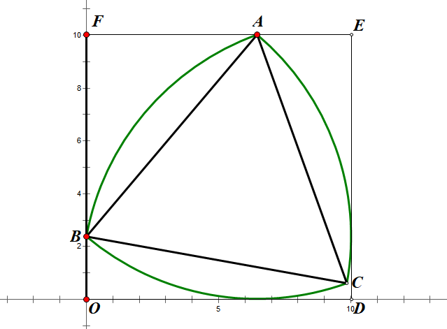And so on, the second, third and fourth situation (shown in Figure 5) can all be worked out using the same principles.

Figure 5. The second, third and fourth situation.

In the second situation, the coordinate of the centre point is:

\( (1-\frac{\sqrt[]{3}}{6}t-\frac{1}{2}\sqrt[]{1-{t^{2}}}, 1-\frac{1}{2}t-\frac{\sqrt[]{3}}{6}\sqrt[]{1-{t^{2}}}) \) (14)

In the third situation, the coordinate of the centre point is:

\( (\frac{\sqrt[]{3}}{6}t+\frac{1}{2}\sqrt[]{1-{t^{2}}}, 1-\frac{1}{2}t-\frac{\sqrt[]{3}}{6}\sqrt[]{1-{t^{2}}}) \) (15)

In the fourth situation, the coordinate of the centre point is:

\( (\frac{1}{2}t+\frac{\sqrt[]{3}}{6}\sqrt[]{1-{t^{2}}}, \frac{\sqrt[]{3}}{6}t+\frac{1}{2}\sqrt[]{1-{t^{2}}}) \) (16)

In addition, in all these situations the domain of t is \( [\frac{1}{2}, \frac{\sqrt[]{3}}{2}] \) .

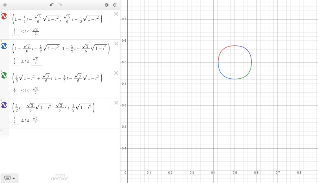
Figure 6. Trail shown by the graph calculator DESMOS.

If we input the parametric function into the graph calculator, we would get a graph shown in Figure 6.

Overall, the center locus of the Reuleaux triangle when it rotates in a square has been successfully expressed by parametric functions and the exact image of its trail is shown in Figure 6.

5. A study about the Reuleaux triangle rotating on a straight line

We already know that the Reuleaux triangle has a constant width, but it is obvious that when it rotates on a straight line, the motion trail of the centre point of the Reuleaux triangle would not maintain on a straight line because the perpendicular distance between the centre point and the ground is not constant. Thus it is worth studying about the exact centre locus of the Reuleaux triangle when it is rotating, and whether the result would match a sort of specific function.

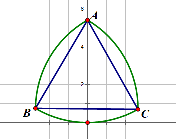Figure 7. The x-axis is tangent to the Reuleaux triangle at the original point.

We would set the Reuleaux triangle’s length of the inner triangle as 1 then we would start rotating clockwise to the right from the situation shown in figure 7. The whole process is to study a complete period of its movement and would be divided into three certain parts: the situation when the x-axis is tangent to the arc BC, the situation when point C is on the x-axis, and the situation when the x-axis is tangent the arc AC.

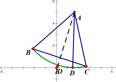Figure 8. The first situation while the Reuleaux triangle is rotating on the x-axis.

Figure 8 shows the first situation when the x-axis is tangent to the arc BC at point D, two other arcs that the x-axis is not tangent to would be omitted to make the figure clearer. We assume that the distance the triangle has traveled is t, which means OD is equal to t, thus it can be concluded that the angle DAE is equal to t in radians as the value of the angle equals the ratio of the length of the arc and the radius. In addition, it is easy to learn that the coordinate of point A is \( (t, 1) \) , as the angle DAE is equal to t, and AE is the angular bisector of the angle BAC, the value of angle CAD would be \( \frac{π}{6}-t \) .

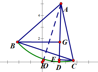Figure 9. The first situation in which lines BG and CF are set.

Then we can construct CE perpendicular to line AD and they intersect at point E (as shown in Figure 9), and therefore the length of CE equals to \( sin{(}\frac{π}{6}-t \) ) and AD equals to \( cos{(\frac{π}{6}-t)} \) . Thus the coordinate of point C is

\( (t+sin{(}\frac{π}{6}-t), 1-cos{(\frac{π}{6}-t))} \) (17)

In addition, the coordinate of B would be

( \( t-cos{(\frac{π}{3}-t), 1-sin{(}\frac{π}{3}-t))} \) (18)

The reason is the same as point A. Hence the coordinate of the centre point of the triangle can be worked out by calculating the average value of the three coordinates of the three vertexes of the triangle.

\( Horizontal ordinate=\frac{1}{3}×[3t+sin{(}\frac{π}{6}-t)-cos{(\frac{π}{3}-t)]} \)

\( =\frac{1}{3}×[3t+\frac{1}{2}cos{t}-\frac{\sqrt[]{3}}{2}sin{t}-\frac{1}{2}cos{t}-\frac{\sqrt[]{3}}{2}sin{t}] \)

\( =t-\frac{\sqrt[]{3}}{3}sin{t} \) (19)

\( Vertical ordinate=\frac{1}{3}×[3-cos{(\frac{π}{6}-t)}-sin{(}\frac{π}{3}-t)] \)

\( =\frac{1}{3}×[3-\frac{\sqrt[]{3}}{2}cos{t}-\frac{1}{2}sin{t}-\frac{\sqrt[]{3}}{2}cos{t}+\frac{1}{2}sin{t}] \)

\( =1-\frac{\sqrt[]{3}}{3}cos{t} \) (20)

Thus the equation of locus of the centre point of the Reuleaux triangle can be expressed as

\( (t-\frac{\sqrt[]{3}}{3}sin{t} \) , \( 1-\frac{\sqrt[]{3}}{3}cos{t} \) ) (21)

As for the second situation(as shown in figure 10), the vertex of the triangle point C, would be on the x-axis as the graph on the right shows, and the triangle would rotate around point C until line BC is perpendicular to the x-axis. We may first mark the centre point of the triangle with the letter i. In this situation, we can first mark out the centre point of the triangle and connect the line between C and i.

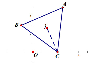Figure 10. The second situation while the Reuleaux triangle is rotating on the x-axis.

In addition, it is easy to discover that point we is just moving on the circle with the equation:

\( {(x-\frac{π}{6})^{2}}+{y^{2}}=\frac{1}{3} \) （22）

The domain of the function is \( [\frac{π-\sqrt[]{3}}{6},\frac{π+\sqrt[]{3}}{6}]. \)

During this process, the triangle would rotate \( 60° \) in total and the ending point is shown in Figure 11. If the movement of rotating goes on, the x-axis would always be tangent to the arc AC.

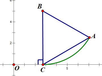Figure 11. The end of the process of the second situation.

As for the third situation(shown in figure 11), in which the x-axis is tangent to the arc AC at point E, we assume that the distance the triangle has passed in this situation is \( θ \) , which means the length of DE is \( θ \) and the value of the angle CBE is \( θ \) in radians.

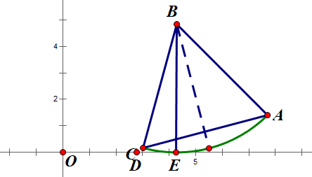Figure 12. The third situation while the Reuleaux triangle is rotating on the x-axis.

Then it is obvious that the coordinate of point B is \( (\frac{π}{6}+θ, 1) \) (shown in Figure 12).

To work out the coordinates of point A and C, we set line CM and AN both perpendicular to BE, and their foot of perpendicular are M and N respectively(shown in Figure 13).

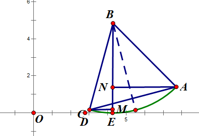Figure 13. The third situation in which lines AN and CM are set.

As we know that the value of the angle is \( θ \) , the length of CM and BM can be expressed using trigonometric functions:

\( CM=sin{θ} \)

\( BM=cosθ \)

Thus the coordinate of point C can be worked out:

\( (\frac{π}{6}+θ-sinθ, 1-cosθ) \) (23)

As the value of angle ABN can be expressed as \( \frac{π}{3}-θ \) , the length of AN and BN can be expressed using trigonometric functions:

\( AN=sin(\frac{π}{3}-θ) \)

\( BN=cos(\frac{π}{3}-θ) \) (24)

Thus the coordinate of point A can be worked out:

\( [\frac{π}{6}+θ+sin(\frac{π}{3}-θ), 1-cos(\frac{π}{3}-θ)] \) (25)

Now we can calculate the coordinate of the centre point of the triangle:

\( Horizontal coordinate=\frac{1}{3}×[3×\frac{π}{6}+3θ-sinθ+sin(\frac{π}{3}-θ)] \)

\( =\frac{1}{3}×[\frac{π}{2}+3θ-sinθ+\frac{\sqrt[]{3}}{2}cosθ-\frac{1}{2}sinθ] \)

\( =\frac{π}{6}+θ+\frac{\sqrt[]{3}}{6}cosθ-\frac{1}{2}sinθ \) (26)

\( Vertical coordinate=\frac{1}{3}×[3-cosθ-cos(\frac{π}{3}-θ)] \)

\( =\frac{1}{3}×[3-cosθ-\frac{1}{2}cosθ-\frac{\sqrt[]{3}}{2}sinθ] \)

\( =1-\frac{1}{2}cosθ-\frac{\sqrt[]{3}}{6}sinθ \) (27)

Thus the equation of locus of the centre point of the Reuleaux triangle in the third situation is:

\( (\frac{π}{6}+θ+\frac{\sqrt[]{3}}{6}cosθ-\frac{1}{2}sinθ, 1-\frac{1}{2}cosθ-\frac{\sqrt[]{3}}{6}sinθ) \) (28)

Overall, the equation of locus of the centre point of the Reuleaux triangle of a certain period (which is \( \frac{π}{3} \) in length) during the whole process of movement has been successfully deduced(shown in Figure 14). Apart from that, it is obvious that the expression is a kind of piecewise function instead of a certain type of function.

This approach just studied a certain period of the equation of locus by working out the expression of the piecewise functions in the period so that the equation of locus of the whole function could be expressed.

Figure 14. The centre locus of the Reuleaux triangle when it rotates on a straight line.

6. Method to construct a stable Reuleaux triangle-shaped wheel

As the equation of locus of the centre point of the Reuleaux triangle when it rotates on a straight line has already been worked out, it would be easy to work out a way to stabilize a car with Reuleaux triangle-shaped wheels.

We still assume that the length of the radius of the circles used to construct the Reuleaux triangle is 1.

Then as the result has already been demonstrated in the former part, a total period would be \( \frac{π}{3} \) in length, therefore we would first transfer the period into a common expression and use the expression to solve the problem.

The expression of the centre point of the Reuleaux triangle would be:

\( (t-\frac{\sqrt[]{3}}{3}sin{t} \) , \( 1-\frac{\sqrt[]{3}}{3}cos{t} \) )

\( {(x-\frac{π}{6})^{2}}+{y^{2}}=\frac{1}{3} \)

\( (\frac{π}{6}+θ+\frac{\sqrt[]{3}}{6}cosθ-\frac{1}{2}sinθ, 1-\frac{1}{2}cosθ-\frac{\sqrt[]{3}}{6}sinθ) \) (29)

In the expressions below,

\( tϵ[0+\frac{π}{3}k, \frac{π-\sqrt[]{3}}{6}+\frac{π}{3}k), \)

\( xϵ[\frac{π-\sqrt[]{3}}{6}+\frac{π}{3}k,\frac{π+\sqrt[]{3}}{6}+\frac{π}{3}k], \)

\( θϵ(\frac{π+\sqrt[]{3}}{6}+\frac{π}{3}k, \frac{π}{3}+\frac{π}{3}k], \)

\( kϵZ. \) (30)

As we have already assumed that the radius of the identical circles used to construct the Reuleaux triangle is 1, which means the length of the constant width of the Reuleaux triangle is 1. Then we can subtract the vertical coordinates of the functions from the length of the constant width 1 so that the distance between the centre point of the Reuleaux triangle and the upper side of the constant width which is parallel to the x-axis can be calculated.

For the first situation:

\( Distance1=\frac{\sqrt[]{3}}{3}cos{t} \)

\( tϵ[0+\frac{π}{3}k, \frac{π-\sqrt[]{3}}{6}+\frac{π}{3}k) \) (31)

As for the second situation, let us first express y using x as a variate:

\( y=\sqrt[]{\frac{1}{3}- {(x-\frac{π}{6})^{2}}} \)

\( Distance2=1-y=1-\sqrt[]{\frac{1}{3}- {(x-\frac{π}{6})^{2}}} \)

\( xϵ[\frac{π-\sqrt[]{3}}{6}+\frac{π}{3}k,\frac{π+\sqrt[]{3}}{6}+\frac{π}{3}k] \) (32)

When it comes to the third situation, the distance is:

\( Distance3=\frac{1}{2}cosθ+\frac{\sqrt[]{3}}{6}sinθ \)

\( θϵ(\frac{π+\sqrt[]{3}}{6}+\frac{π}{3}k, \frac{π}{3}+\frac{π}{3}k] \) (33)

Till now we have already worked out the length needed to balance out the movement, then we are able to design a construction of mechanism which is connected to the axle of the Reuleaux triangle-shaped wheel. Therefore the mechanism can move up and down repeating a certain period in order to make the distance between the ground and the bottom of the car always the same, thus the car can be stabilized.

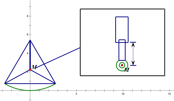
Figure 15. The starting situation of the construction.

Figure 15 shows the situation while the construction is at its status of maximum vertical length. As the wheel starts rotating, the vertical length would gradually decreases until it reaches the status of minimum vertical length shown in Figure 16.

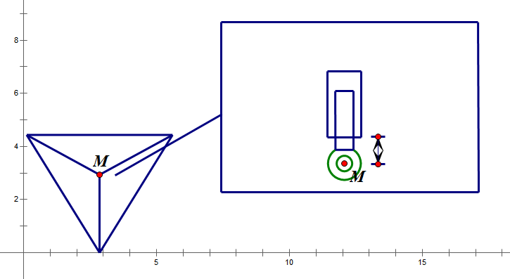Figure 16. The situation when the vertical length of the construction is the shortest.

Till now half of the whole period has been completed, and the vertical length of the construction would generally increase until it reaches the end point of the process(As shown in figure 17).

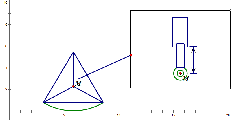Figure 17. The ending situation of the whole period.

In conclusion, this approach has offered a practicable method of designing a mechanism to stabilize a car with Reuleaux triangle-shaped wheels.

7. Approaches of drawing constant width curves

We already know that the Reuleaux triangle belongs to constant width curves, then we may be concern about what may other constant width curves look like and whether there is a certain approach to drawing them. This inspiration comes from the paper studying constant width curve written by Horst Martini[3]. The following content of the paper would mainly introduce and demonstrate an approach to drawing constant width curves. As constant width curves can be constructed using mutually intersecting lines and there is a certain rule inside[4-5]. Firstly, let’s introduce a basic element of this approach as it would be used through the whole approach.

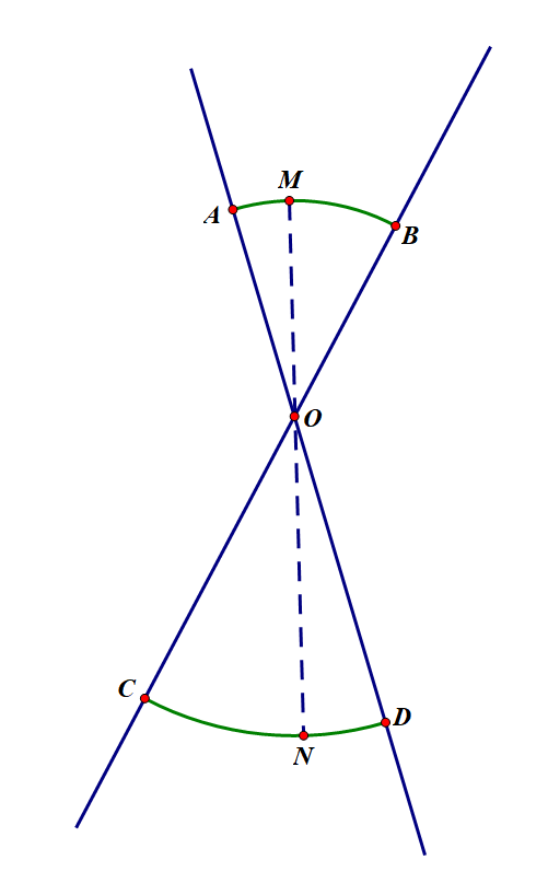Figure 18. Two arcs constructed by two intersecting lines.

As it is shown in figure 18, arc AB and arc CD are formed by two intersecting lines, and the radius angles they correspond to are of the same value. We can easily find that the length of OA and OB are the same as they are both radius to the same circle, and it is the same to OC and OD. Thus we can learn that the length of AD is equal to that of BC as point O is the intersecting point of lines AD and BC. Furthermore, any line like AB and CD that goes through point O and has its two vertexes on the arc AB and CD respectively has a fixed length. Take MN for example, its length is equal to that of AD and BC’s. Hence the arcs AB and CD somehow have a constant width.

We first draw three mutually intersecting lines AB, CD and EF.

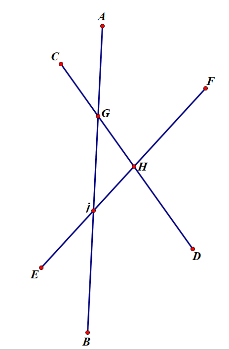Figure 19. Three mutually intersecting straight lines.

Then we can draw an arc A1C1 whose centre of the circle is point G, then we choose point H as centre of the circle and let HC1 be the radius to draw the arc C1E1. We then select We as the centre of the circle, IE1 as radius and draw the arc E1B1. With the same principle, we can complete the later work until the a complete curve forms as Figure 19 shows.

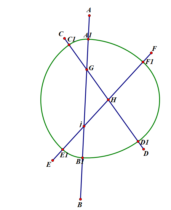Figure 20. The complete curve based on three mutually intersecting lines.

In this situation(see figure 20), we can easily demonstrate that the curve is a constant width curve using the principle we proved previously of this part. We can count that three intersecting points have been used as the centre of the circle. The rule we choose for the centre of each circle is that the two neighbor arcs may both have one of their radius on the same line. For example, in the former situation, after having drawn the arc A1C1, its radius was GC1, the next arc we drew was C1E1 and its radius was HC1, GC1 and HC1 are both on the line CD. As we have already proved in the beginning, we can ensure that when we draw the arc A1C1 and B1D1, A1B1 is equal to C1D1, and for the same reason C1D1=E1F1, thus A1B1=C1D1=E1F1, which means the curve we get is a constant width curve. Apart from that, on each line there are always two points that are used as the centres of circle. Then we may consider about the situation which is based on four mutually intersecting lines.

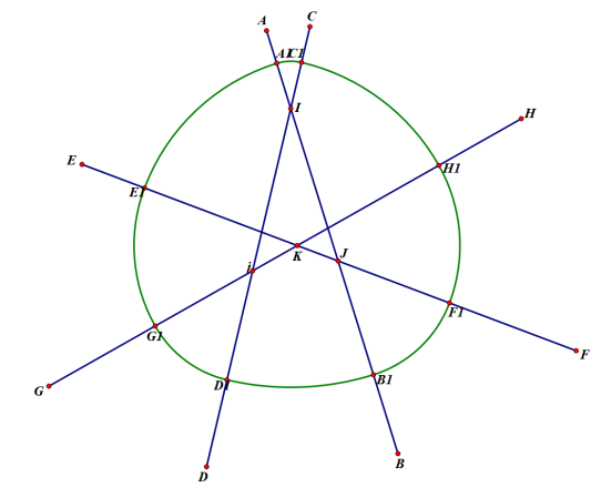Figure 21. The constant width curve based on four mutually intersecting lines.

In this situation(as shown in figure 21), four points I, i, J, and K have been used as the centres of the circles and a new constant width curve has been successfully drawn. In addition, there are always two points that are chosen to be the centres of circles. Till now we may realize that there must be a rule in drawing this figure, thus we may keep on adding the number of lines.

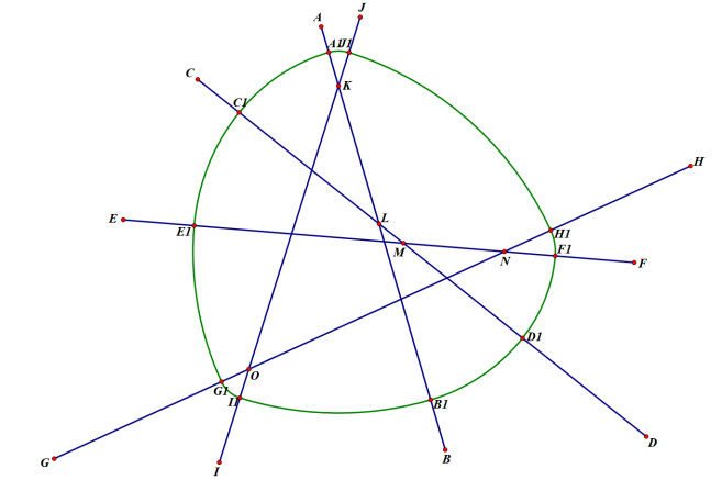
Figure 22. The constant width curve based on five mutually intersecting lines.

As we can observe in Figure 22, there are 5 intersecting points that used to be the centres of circles. Moreover, like the former two situations, there are also two points on each line that are used to be the centres of circles.

Now we can assume that, no matter how many mutually intersecting lines are constructed, a certain constant width curve can always be drawn. In addition, there are always two points on each line that are chosen to be the centres of circles. However, this problem can not be solved by mathematical induction easily as we can not imagine or construct the situation in which there are n mutually intersecting lines. (n is a positive integer) Thus we may study about the situations in which there are 6 and 7 mutually intersecting lines.

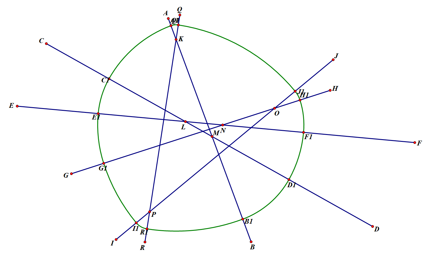
Figure 23. The constant width curve based on six mutually intersecting lines.

After observing Figure 23, we can conclude that the number of points used as centres of the circle is equal to the number of straight lines. In addition, on each line we can always find two points that have been used as centre of circles. As a result, this conclusion can be used in all possible situations so that we can draw any constant width curve using mutually intersecting lines.

8. Conclusion

Overall, the paper has introduced and demonstrated several features of the Reuleaux triangle and has given some feasible uses. To be more specific, the paper introduced a clear way to demonstrate that the Reuleaux triangle has a constant width and then used analytic geometry and differentiation to prove it rigorously. Then the paper used properties of polar form and Euler form of complex numbers to work out the movement of the triangle as it rotates in a square and used parametric functions to express the centre locus of the Reuleaux triangle. In addition, the paper has also worked out the centre locus of the Reuleaux triangle as it rotates on a straight line using trigonometric functions and worked out the exact graph of the trail. Thus the feasible mechanism construction to stabilize a car with Reuleaux triangle-shaped wheels has been successfully introduced this part is based on the former proof. To develop the idea of ‘constant width’, the paper has introduced and demonstrated an approach to drawing constant width curves based on mutually intersecting straight lines. However, due to the restriction of the knowledge We have acquired, We have only used the method of finding the law rather than mathematical induction.

Though the demonstrations and proofs have already been accomplished, we should still consider whether practical approaches would be beneficial in real life. Taking Reuleaux triangle-shaped wheels for example, though it has been proved that the method is practicable and a mechanism construction has been introduced, this approach would consume extra energy when compared with normal wheels. Thus it is hard to be applied to real life. By contrast, the idea of Reuleaux triangle-shaped drills is much better, as it has already been used in industrial production in many regions. However, this paper only demonstrated the trail of the centre point as it rotates, the relationship between the size of the triangle and the size of arcs at the corners of the square has not been studied yet.

For the topic of Reuleaux triangle, there are still a number of regions that have not been studied or discovered. For example, the question of whether the curve formed by identical circles is always a constant width curve is worth studying. Apart from that, the Reuleaux triangle may be able to replace the balls inside the bearings so that it can be applied in many industrial regions. As a result, there are still many secrets inside the Reuleaux triangle and they are waiting for us to discover and study about.

References

[1]. Javier Barrallo,An introduction to the Vesica Piscis, the Reuleaux triangle and related geometric constructions in modern architecture. 2015. https://link.springer.com/article/10.1007/s00004-015-0253-9
[2]. Mikhail Razumov, Stress calculation of moment transmitting roll with profile on the base of Reuleaux triangle. .2014. https://www.metaljournal.com.ua/assets/Archive/en/MMI3/10.pdf
[3]. Horst Martini. A new construction of curves of constnant width. 2008 https://www.sciencedirect.com/science/article/abs/pii/S0167839608000745
[4]. Bruce B. Peterson. Intersection properties of curves of constant width. 1971 https://projecteuclid.org/journals/illinois-journal-of-mathematics/volume-17/issue-3/Intersection-properties-of-curves-of-constant-width/10.1215/ijm/1256051608.pdf
[5]. Stanley Rabinowtz. A polynominal curve of constant width. 1997 https://projecteuclid.org/journalArticle/Download?urlId=10.35834%2F1997%2F0901023
Cite this article
Wei,M. (2023). The Secrets inside the Astonishing Reuleaux Triangle and its Practicable Uses. Theoretical and Natural Science,5,368-385.
Data availability
The datasets used and/or analyzed during the current study will be available from the authors upon reasonable request.
Disclaimer/Publisher's Note
The statements, opinions and data contained in all publications are solely those of the individual author(s) and contributor(s) and not of EWA Publishing and/or the editor(s). EWA Publishing and/or the editor(s) disclaim responsibility for any injury to people or property resulting from any ideas, methods, instructions or products referred to in the content.
About volume
Volume title: Proceedings of the 2nd International Conference on Computing Innovation and Applied Physics (CONF-CIAP 2023)
© 2024 by the author(s). Licensee EWA Publishing, Oxford, UK. This article is an open access article distributed under the terms and
conditions of the Creative Commons Attribution (CC BY) license. Authors who
publish this series agree to the following terms:
1. Authors retain copyright and grant the series right of first publication with the work simultaneously licensed under a Creative Commons
Attribution License that allows others to share the work with an acknowledgment of the work's authorship and initial publication in this
series.
2. Authors are able to enter into separate, additional contractual arrangements for the non-exclusive distribution of the series's published
version of the work (e.g., post it to an institutional repository or publish it in a book), with an acknowledgment of its initial
publication in this series.
3. Authors are permitted and encouraged to post their work online (e.g., in institutional repositories or on their website) prior to and
during the submission process, as it can lead to productive exchanges, as well as earlier and greater citation of published work (See
Open access policy for details).