1. Introduction

1.1. Background

Ocean is a complex system that is mainly stably density stratified; i.e., the water at the bottom has a larger density than the water on the top. The density of seawater is affected by temperature and salinity leading to density differences in both vertical and horizontal directions. For example, after basking in the sunshine, the salinity of the water will increase due to water evaporation. Such a phenomenon is typical in tropical and subtropical regions leading to the salinity on the top of the ocean being higher than the bottom of the ocean. Another example of salinity difference is near the estuary, where the freshwater of the river is on top of the salty water of the sea. Moreover, when the relatively salty water of the Mediterranean Sea is injected into the relatively fresh water in the Atlantic Ocean, it also leads to the salinity difference between the top and bottom. The temperature difference of seawater in the vertical direction can be induced by the sunshine, particularly near the tropical region. In the polar region, the top glacier also leads to a lower water temperature than the ocean bottom. Under the condition of uneven distribution of temperature and salinity both contributing to the density difference, the phenomenon of double diffusion convection in the ocean will occur. The double-diffusive convection includes both salt-finger convection (hot salty water on top of cold fresh water) and diffusive convection seawater (cold fresh water on top of hot salty water). This work focuses on salt-finger convection.

1.2. Literature review

Salt-finger convection is presented in different parts of the ocean where warm salty water overlies cooler fresher water, which is widely observed in tropical oceanography measurement. As Turner [1] has mentioned, flow in salt-finger regime is drawing on the potential-energy supply in the salinity distribution and will continue so long as this is renewed by evaporation at the sea surface. The Caribbean-Sheets and Layers Transect (C-SALT) field program offered in Schmitt et al. [2] showed layers in spring and autumn of 1985 in Barbados, tropical Atlantic, where salt-finger convection is favoured. These authors found that vertical movement of salt fingers made a major contribution to mixing in the main thermocline regions. In addition, Tait and Howe [3] confirmed the existence of double diffusion in coastal oceanic regions. Padman and Dillon [4] used thermal microstructure data from the Canada Basin and found that shear instabilities driven by the internal wave field may significantly modified by multiple factors.

Salt-finger instability is driven by the diffusivity difference between salt and temperature, even though the overall density is in a top-light and bottom-heavy configuration (stable stratification). The molecular diffusivity of salt in seawater is much smaller than that of heat. With an overall stable stratification, the warm, salty water floats on top because it is slightly less dense than cold, fresh water. As the warm, salty water loses heat faster because the temperature diffusivity is much larger than salt, it becomes denser and moves further downward [5].

One important response parameter of salt-finger convection is the horizontal length scale (finger width), which will determine the length scale employed in the parameterization of ocean modelling. To investigate the width of salt fingers, we can use visualization of a vertical plane in the tank by mixing colouring dyes with hot salty water and mixing it fluorescent dye into the upper layer by an argon-ion laser. Shirtcliffe and Turner [6] used a shadowgraph system to visualize the planform of salt-sugar fingers and found that the fingers tended to be square with the correlation in the orientation of neighbouring fingers extending over several finger widths. Furthermore, Yang et al. [7] employed a three- dimensional direct numerical simulation to analyse the finger width within a bounded domain and obtained the scaling law of finger width over density ratio. Stern et al. [8] suggested that the finger width that maximizes the buoyancy flux is being selected, and once a finger width is chosen, the flux would be determined for a given constant value of salinity and temperature gradient. Collective instability [9] indicates that the amplitude of the fastest-growing fingers is limited by the instability of the fingers.

In our experiment, we decide to examine how the different density ratios may affect the linear instability of salt fingers. A three-dimensional linear stability analysis is carried out for a convection layer in which both the temperature and solute distributions are linear in the vertical direction. Stability theory is involved during the process of exploring salt fingers inferred from the hot salty water convection experiment [10]. The experiment is going to be concentrated on the unstable mode with its growth rate. Accordingly, Shen [11] found that as the fingers evolved the velocity gradient spectrum broadened as energy was transferred to lower wavenumbers. Although the computations by Shen [11] had lower values of the Prandtl number ( \( Pr \) = 1 or 2) and diffusivity ratio ( \( τ \) = 0.1 or 0.2) was higher than in the heat-salt system ( \( Pr \) = 7, \( τ \) = 0.01), it is unlikely that the overall evolution of the spectrum should depend on the exact values of these parameters.

Staircases have also been widely observed in the oceanography measurement in the salt-finger regime [2,3,5,12,13], which shows several well-mixed (uniform in vertical) region separated by the sharp interface (large gradient in vertical) in both temperature and salinity. Furthermore, staircases have been observed in both direct numerical simulations [14–17] and laboratory experiments [18,19]. Radko [14] proposed a \( γ \) instability mechanism that predicts the staircase based on the onset of horizontal averaged modes with certain parameterization of the heat flux and salinity flux. One indication of the staircase is based on the horizontal velocity, where a non-zero horizontal velocity indicates the potential presence of staircases, while vertical velocity is typically associated with the mixed region.

One important measurement of the intensity of the finger is vertical velocity. Taylor and Bucens [20] used the fluxes calculated based upon the model in order to derive vertical temperature and salinity profiles through the finger zone. During their experimental procedure, they filled the tank to a depth of 210 mm with filtered tap water before heated to the desired upper layer temperature. it not only illustrates a method for the inquirer to clearly visualize the fingerprints in the water but also provides a good idea of the depth of the water, which inspires further experimental analysis of salt-finger convection.

1.3. The present work

This work designed homemade experiments to investigate salt-finger convection. The experiment is done by pouring a designated concentration of salty hot water into the tank that contains a fixed amount of fresh, cold water. The temperature difference is fixed and the concentration of salty water (salinity) is varied leading to different density ratios. A lower density ratio corresponds to a larger salinity difference between the top and bottom layer showing a stronger destabilizing effect. salt fingers are visualized by dye and their displacement over time is obtained by recording using a camera and analysing video using Tracker. These experiments effectively generate the phenomena resembling salt-finger micro-structure in the ocean.

This paper is going to explore the concepts of finger width, the velocity of salt-finger convection through both experimental data and linear stability analysis. We can compare the result of different density ratios by examining the trends that are led by the salinity level of the salty hot water being added. The vertical and horizontal characteristic velocities of salt fingers are obtained from experiments over different density ratios. Finger widths over a range of density ratios obtained from the experiments are compared with that predicted from the linear stability analysis.

The remainder of this paper is organized as follows. §2 defines the key concept of governing parameter of salt-finger convection and linear stability. Then, section 3 describes the experiment, its setup, procedure, and accuracy, and section 4 presents results obtained by tracking salt fingers. Section 5 then compares the result of my experiment with the result obtained by linear stability analysis and studies in the literature. We conclude this paper and discuss potential future work in §6.

2. Governing parameter of salt-finger convection

In this section, we describe governing parameters of double-diffusive convection [10]. The diffusivity ratio

\( τ=\frac{{κ_{S}}}{{κ_{T}}} \) (1)

refers to the ratio between salinity diffusivity \( {κ_{S}} \) and temperature diffusivity \( {κ_{T}} \) . The Prandtl number

\( Pr=\frac{ν}{{κ_{T}}} \) (2)

is the ratio between kinematic viscosity \( ν \) and the thermal diffusivity \( {κ_{T}} \) . The kinematic viscosity \( ν \) can be also understood as the diffusivity of momentum and thus it also measures the rate of diffusivity between momentum and temperature.

We also select the vertical water height \( H \) as a characteristic length scale to define a thermal Rayleigh number:

\( R{a_{T}}=\frac{∆ρ{H^{3}}g}{v{ρ_{w}}{κ_{T}}} \) (3)

where \( ∆ρ \) is the density difference between the top and bottom due to thermal stratification, \( g \) is the gravity and \( {ρ_{w}} \) is the density of water.

Here, we consider the equation of state as linear and the density is influenced by both temperature and salinity \( ({ρ_{*}}- {ρ_{r*}})/{ρ_{r*}}=-α({T_{*}}- {T_{r*}})+ β({S_{*}}- {S_{r*}}) \) . Here, a subscript \( * \) indicates a dimensional variable. \( α \) and \( β \) are thermal expansion coefficient and salinity contraction coefficient, respectively. Thus, another governing parameter of salt-finger convection is the density ratio

\( {R_{ρ}}=\frac{α∆T}{β∆S} \) (4)

which measures the degree of contribution to the density variation between temperature and salinity gradients of the fluid.

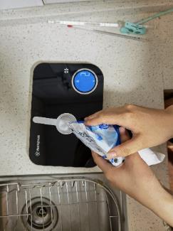
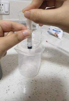
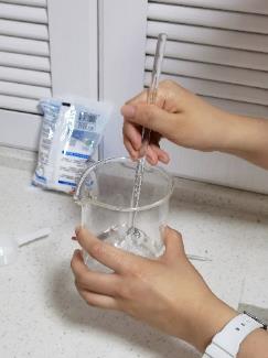
(a) (b) (c)

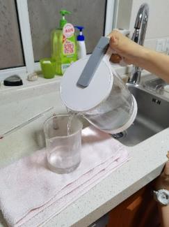
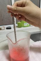
Figure 1. Example procedure to obtain the designed concentration of salt using dilution method. Panel (a) measures 2 g of salt added to 100 g water with ≈20 PSU, panel (b) obtains 10 g of salty water with 20 PSU and then adds hot water until it is cooled down to 75 ℃, and panel (c) stirring the salty water to obtain well-mixed hot salty water with 2 PSU and 75 ℃.

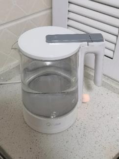
(a) (b)

Figure 2. Example procedure to obtain hot boiling water. Panel (a) is boiling 250 ml of water is being electronically heated to boil in the thermos bottle, and panel (b) is adding the beaker, which holds the salty water, up to 100 ml.

In this work, we analyse the temperature and salinity that influence the water density, and thus, we fix \( Pr \) = 7 and \( τ \) = 0.01. The density ratio will be modified based on the salinity of the top water that is added in the experiments.

3. Experimental setup

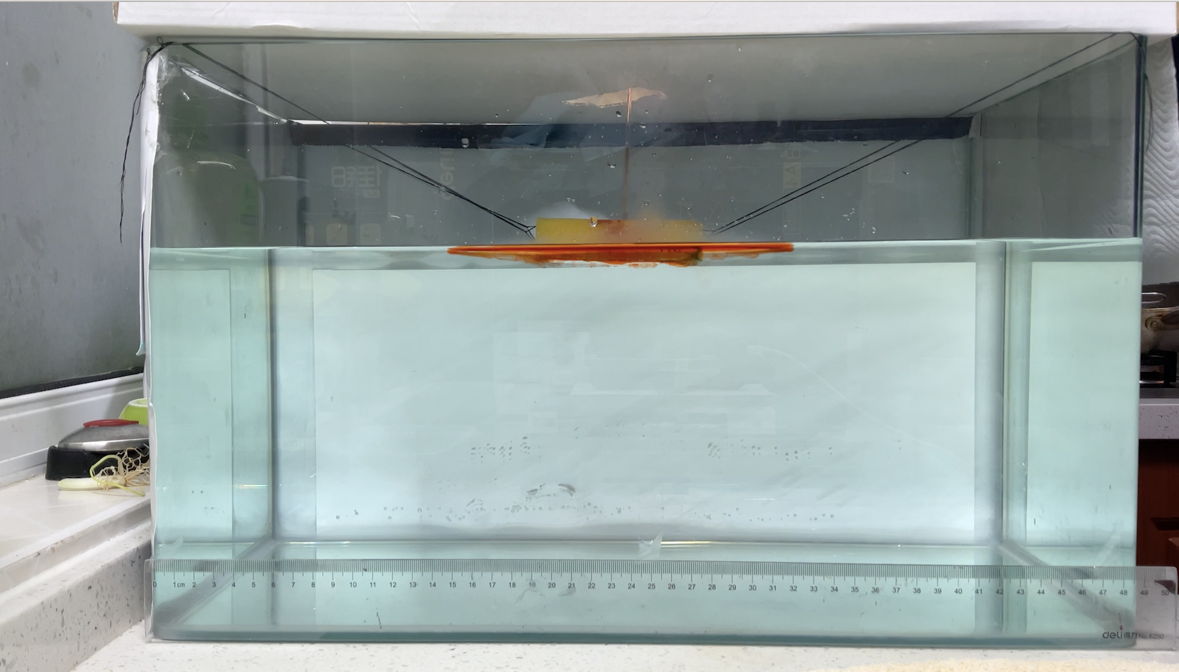
A total of three experiments are conducted to explore salt-finger convection through observation. There are eight trials of the experiments being taken, while the mass of the salt being added is the independent variable. The apparatus being used are: a large deep-water tank, a stir rod, colourful pigment, a sponge, cold clean water, a large beaker, thermometer, ruler, and needle tubing. This experiment is separated into four procedures: preparation, titration method, obtaining the hot salty water, and pouring the water into the tank. The water tank is rectangular of 50 cm (length) × 27 cm (width) × 30 cm (height). The experimental measurement is focused on the plane with 50 cm × 30 cm.

(a) (b)

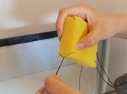
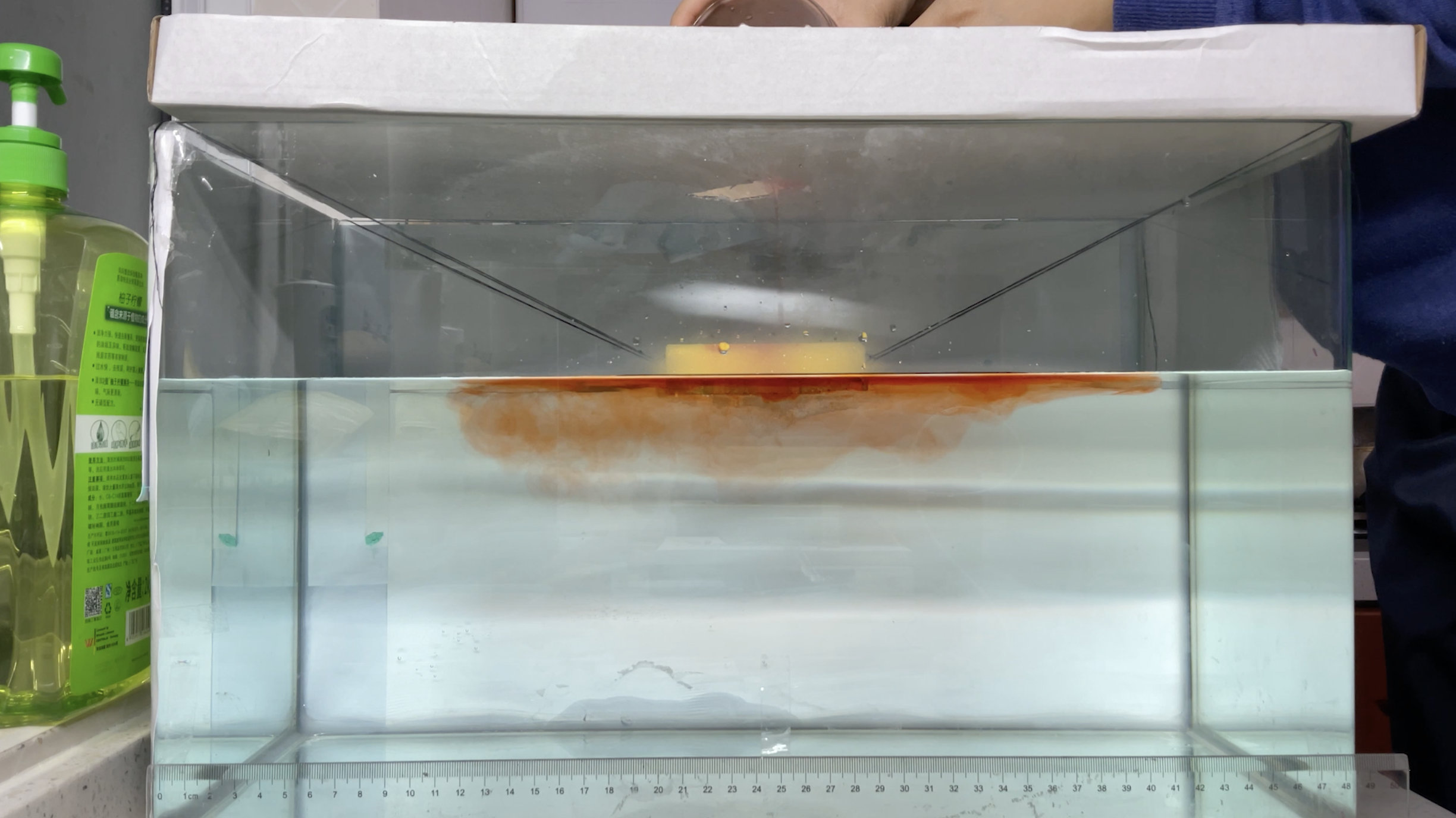
Figure 3. Detailed experimental procedure to ensure the accuracy of the experiment. Panel (a) is reading the mercury at right angle to scale, in order to ensure that the temperature of the hot water is in control. Panel (b) is passing a thread through the sponge and fixes the thin string in the sponge. This allows me to fix the sponge around the middle of the water tank, rather than flowing around on the surface of the water.

(a) (b)

Figure 4. Example procedure to pour the hot salty water with dye into the tank. The pouring process lasts around 10 s. Panel (a) is pouring hot salty water with dye (75 ℃, 0.5 PSU), while panel (b) is pouring hot salty water with dye (75 ℃, 1 PSU).

(a) (b)

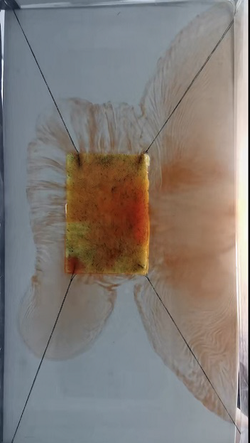
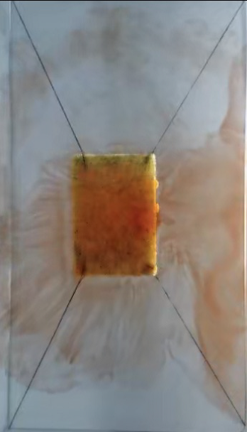
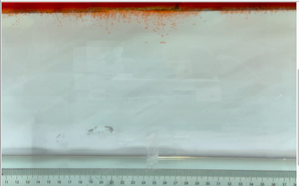
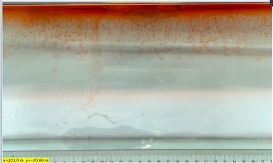
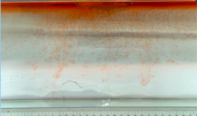
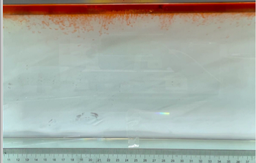
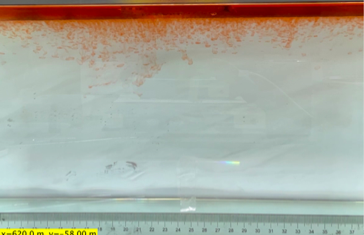
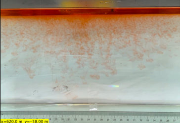
Figure 5. Visualization from the bottom of the tank, exploring the phenomenon happens opposite to the surface of the water.

In the experiment, the volume of the hot water, cold fresh water, the temperature of both water and the type of salt being added are fixed. The mass of salt being added is to be varied to analyse the effect of different density ratios. Then phenomenon occurs after different masses of salt are mixed in the hot water and added to the cold fresh water. To start an experiment, the tank is filled to a depth of 20 cm with 22 ℃ of cold fresh water. When the set depth of the water is reached, the sponge is placed at about the middle of the water surface by tying its four corners with strings and connecting them to the edges of the tank; see Figure 3 and Figure 4.

Then, the specific gram of salt added to the hot water can be obtained using the dilute method (Figures 1-3). After weighing a specific amount of salt with an electronic balance, we add them into the 100ml of warm water. Then, we extract the specific amount of salty water from this beaker to the other clean beaker using needle tubing and fill up the beaker to 100ml with boiling water. The following steps are used for the dilute method in order to obtain the concentration of salt that I need:

• Add 10 drops of edible food colouring into the beaker and stir the solution using a stirring rod. Measure the temperature of the hot water using the thermometer, and ensure that the temperature of the water is 75 ℃.

• Repeat this step to obtain the different masses of salty water, while the numerical values are different.

• During the experiment, when pouring 100ml of hot salty water through the sponge into the water in the tank, the speed of pouring salty water into the tank must maintain constant at a very low valve. Ensure that the approximately average velocity is the same for these experiments.

The dilute method is used to resolve the proportion of salt in the salty hot water. To make the result of the experiment accurate, the temperature of the hot water is needed to be determined. Since the hot water being poured would not be absolutely boiled. Its actual temperature needs to be controlled at 75 ℃, in order to do further calculation and analysis.

The edible pigment is used as a dye. It is used to differentiate the colour of pure water and the solution that is being added. In this experiment, red-orange colour is used, which has clear contrast with the colour of the water. We also measure the density of water with dye and the influence of dye on the density is negligible.

The sponge is used to ensure that the solution is diffused at a slow speed so that the process of double diffusion can be carefully observed. The sponge fixes its position, about the middle of the tank, in order to avoid horizontal motion. Since horizontal motion may cause salt fingers in the water to form irregular shapes or tilt. Here, the sponge is being placed in the middle of the tank by connecting its four edges with a thin string (as shown in the Figure5), so it will not be crushed by the limitation of space on one side of the fingers.

4. Results

We perform eight different groups of experiments with different salinity differences between the top and bottom water, but the temperature difference is fixed. The corresponding parameters and associated density ratio \( {R_{ρ}} \) are summarized in table 1.

Table 1. The temperature and salinity of the top water, the temperature of the bottom water, and the corresponding density ratio for eight different groups of experiments.

Here, we compute the density ratio as

\( {R_{ρ}}=\frac{α∆T}{β∆S}=\frac{a∆T}{b∆S} \) (5)

where we use \( a \) = 0.24 ± 0.1 kg·m⁻³·K⁻¹, and \( b \) = 0.76 ± 0.02 kg·m⁻³·(g·kg⁻¹)⁻¹ [21]. We also compute the thermal Rayleigh number

\( R{a_{T}}=\frac{∆ρ{H^{3}}g}{v{ρ_{w}}{κ_{T}}}=\frac{a∆T{H^{3}}g}{v{ρ_{w}}{κ_{T}}}=4.265×{10^{7}} \) (6)

where \( a \) is the coefficient previously used, \( ∆T \) is the temperature difference between top and bottom, \( H \) is the layer height 20 cm, \( g \) is gravity acceleration, \( ν \) = 1 mm²/s is kinematic viscosity, and \( {κ_{T}} \) = 23.38 (mm²/s) is thermal diffusivity. \( {ρ_{w}} \) is the density of water.

4.1. Visualization and analysis

(a) \( {R_{ρ}} \) = 334.7 (0.005 g)

(b) \( {R_{ρ}} \) = 167.36 (0.01 g)

(c) \( {R_{ρ}} \) = 83.6 (0.02 g)

(d) \( {R_{ρ}} \) = 33.47 (0.05 g)

(e) \( {R_{ρ}} \) = 16.74 (0.1 g)

(f) \( {R_{ρ}} \) = 8.36 (0.2 g)

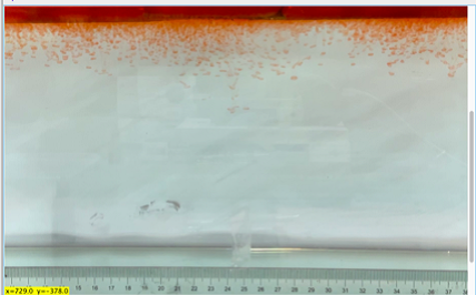
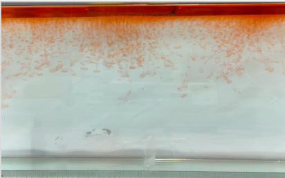
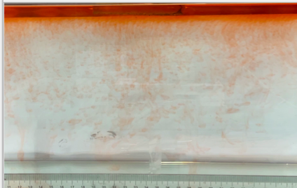
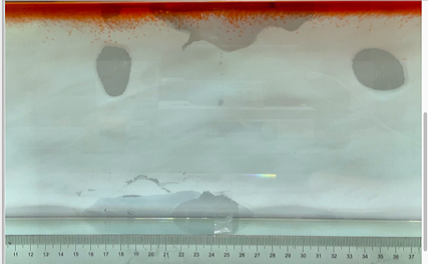
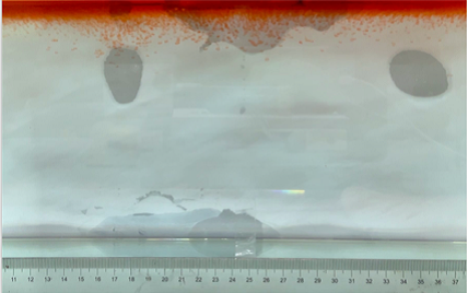
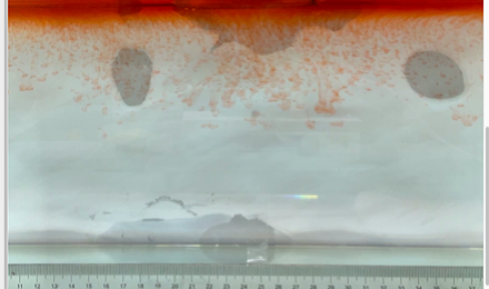
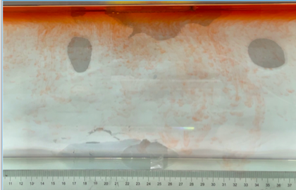
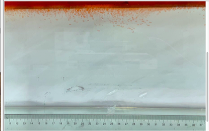
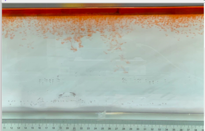
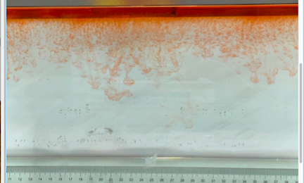
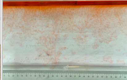
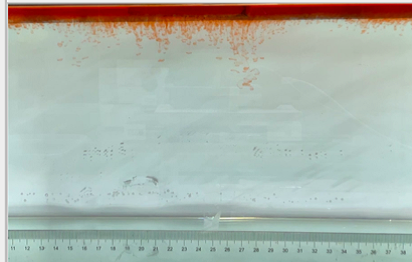
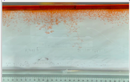
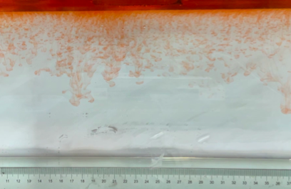
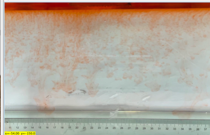
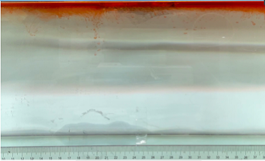
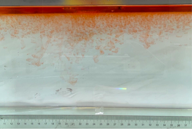
Figure 6. Visualization of salt fingers from experiments associated with six different density ratio \( {R_{ρ}}∈ \) [8.36, 334.7] with salt mass per 100 g water shown in the bracket. Each column corresponds to intervals determined by the average level of salt fingers in the tank.

(a) \( {R_{ρ}} \) = 167.36 (b) \( {R_{ρ}} \) = 83.6

(c) \( {R_{ρ}} \) = 33.47 (d) \( {R_{ρ}} \) = 16.736

(e) \( {R_{ρ}} \) = 8.36

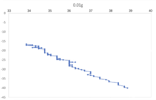
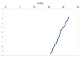
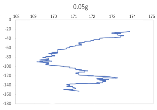
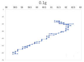
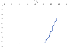
Figure 7. Displacement (mm) of salt fingers associated with different density ratios \( {R_{ρ}}∈ \) [8.36, 167.36].

This work separates each experiment into four intervals based upon direct observation of its phenomenon. In the first stage, six experiments’ salt-finger typesets are similar, and spread uniformly. Starting from the third phase of the experiment, the range of the horizontal and vertical movements varied greatly.

Figure 6 shows the visualized phenomenon of the results for six different masses of salt is added to the water and associated density ratio \( {R_{ρ}}∈ \) [8.36, 334.7]. The four intervals of six different independents experiments depict salt-finger movements during the experiment. For the first interval, six experiments’ salt-finger points are moving with a vertical manner, which does not have large tilts to either left or right. Experiment associated with 0.1 g of salt solution as an exception, where four to five of the salty fingers are moving straight down, which was far past the movement of the other salty fingers. This can be seen as an exception, which might be a random error due to small spoilage of the solution while pouring it down from the top by hand. In the third interval, even though most fingers in all these experiments are moving with a vertical tendency, few of the salty fingers are moving faster, surpassing most of the others, such as the large salty finger shown on the panel of 0.2 g in the third interval. After four fifth of the traveling, in the fourth interval, the position of salt fingers is different over a relatively long distance, some small salt fingers are still located at the second interval, while less than half of them cross more than one-third of the depth of the water. Also, due to the reason that many salt fingers have travelled to the bottom, which is a relatively long distance from the surface, their movements start to tilt to either side of the tank due to the bottom boundary.

4.2. Vertical and horizontal velocity

Using the video taken from the side of the water tank, we record salt fingers every 0.1 seconds, tracking the movement of specific fingers. Then, we use tracker software to obtain the horizontal and vertical position of the finger over different times. We then compute the horizontal and vertical velocity by separating movements into different time domains and then perform a linear regression.

Table 2 provides the mean, variance and skewness of vertical velocity \( w \) and horizontal velocity \( u \) as a function of density ratio \( {R_{ρ}} \) . Here, the skewness function measures the symmetry of the distribution of obtained salt fingers velocity. In the last column, we also report the number of points that are sampled in the recorded video. Note that we select the corresponding time domain that salt fingers under tracking is not merging. Here, we can find that the mean vertical velocity is in general increasing as the density ratio decreases, which is consistent with a stronger destabilizing effect of salinity difference at a lower density ratio. For some results at the high-density ratio, the variance of experimental data is relatively high leading to the violation of this trend. Note that the current ‘run-down’ experimental setup also allows the temperature gradient and salinity gradient to evolve over time but not maintained as a constant. The mean horizontal velocity in table 2 is also not zero, indicating that salt-finger is also moving in the horizontal direction. This is consistent with the trajectory shown in Figure 7.

Figure 7 shows the horizontal displacement ( \( x \) -axis) and vertical displacement ( \( y \) -axis) for five different density ratios, where fingers’ horizontal positions are varying, without specific patterns. Its horizontal movement may change throughout the process of flowing down, to the bottom of the tank. As shown in Figure 7(a), when 0.01 g of the salt was added in the water ( \( {R_{ρ}} \) = 167.36), the \( x \) -axis moved to the left before the two fingers were combined. To notice that the velocity and variance of results associated with 0.5 g 0.02 g and 0.05 g per 100 g water might seem to be abnormal, which is due to the fact that the selected salt fingers are combined during their traveling, which should be negligible.

Experiment error of the average velocity calculation can be also analysed. The velocity of water pouring onto the sponge is one experimental error. During the experiment, the position and gesture of the tester are the same, but the velocity of the water pouring on to the sponge can be differentiated between experiments. Repeating the experiment multiple times and compare videos with different values of the dependent variables, we select the experiments with the trajectory closest to the average trajectory. After the results are selected, we also eliminate the abnormal data points based on the plotted gap. Finger

4.3. Width and height

Estimating the finger width (horizontal wavelength) is also an important question. Here, we select four phrases of salt fingers for six different salinity levels: 0.001 g, 0.005 g, 0.01 g, 0.02 g, 0.05 g, and 0.1 g salt within 100 g water. By averaging three finger widths that is obtained by tracking the fingers’ movement every 20 unit time. The skewness of the six experiments seem to be random, but it is within the expectation for the experiment, since the tilt of the finger may be different due to the acceleration of the fluid being poured into the tank of fresh water. We note that the variation of experiments No. 3 and No. 4 seem to be abnormal compared with the other four experiments because the number of selected points varied due to the movement of salt fingers; i.e., we need to stop tracking the points and start to find the mean and variation.

5. Linear stability analysis

In this section, we perform the linear stability analysis following the procedure in Radko [10, §2]. We firstly decompose the total temperature and salinity as a linear base state and the deviation:

\( {T_{tot}}=z+T \) (7-1)

\( {S_{tot}}=z+S \) (7-2)

Then the governing equation of velocity, temperature and salinity deviation are governed by Navier-Stokes equations with Bousinessq approximation:

\( {∂_{t}}u+u∙∇u=Pr{∇^{2}}u-∇p+PrR{a_{T}}(T-R_{ρ}^{-1}S){e_{z}} \) (8-1)

\( ∇∙u=0 \) (8-2)

\( {∂_{t}}T+u∙∇T+w={∇^{2}}T \) (8-3)

\( {∂_{t}}S+u∙∇S+w=τ{∇^{2}}S \) (8-4)

We recall that length is normalized by the vertical water height \( H \) , velocity is normalized by \( {κ_{T}}/H \) , and time is normalized by \( {H^{2}}/{κ_{T}} \) . Temperature and salinity are respectively normalized by the temperature and salinity difference between the top and bottom layers.

For linear stability analysis, we then dropped the quadratic nonlinear terms to obtain:

\( {∂_{t}}u=Pr{∇^{2}}u-∇p+PrR{a_{T}}(T-R_{ρ}^{-1}S){e_{z}} \) (9-1)

\( ∇∙u=0 \) (9-2)

\( {∂_{t}}T+w={∇^{2}}T \) (9-3)

\( {∂_{t}}S+w=τ{∇^{2}}S \) (9-4)

We can also use the divergence-free constraint in (9b) to eliminate the pressure:

\( {∂_{t}}{∇^{2}}w=Pr{∇^{4}}w+PrR{a_{T}}∇_{⊥}^{2}(T-R_{ρ}^{-1}S) \) (10-1)

\( {∂_{t}}T+w={∇^{2}}T \) (10-2)

\( {∂_{t}}S+w=τ{∇^{2}}S \) (10-3)

where \( \hat{∇}_{⊥}^{2}=∂_{x}^{2}+∂_{y}^{2} \) is horizontal Laplacian operator. We also make the normal mode ansatz in horizontal and vertical directions as

\( [w(x,y,z,t),T(x,y,z,t),S(x,y,z,t)]=[\hat{w}(t),\hat{T}(t),\hat{S}(t)]{e^{i({k_{x}}x+{k_{y}}y+{k_{z}}z)}}+c.c. \) (11)

where \( c.c. \) means complex conjugate

\( {∂_{t}}{\hat{∇}^{2}}\hat{w}=Pr{\hat{∇}^{4}}\hat{w}+PrR{a_{T}}\hat{∇}_{⊥}^{2}(\hat{T}-R_{ρ}^{-1}\hat{S}) \) (12-1)

\( {∂_{t}}\hat{T}+\hat{w}={\hat{∇}^{2}}\hat{T} \) (12-2)

\( {∂_{t}}\hat{S}+\hat{w}=τ{\hat{∇}^{2}}\hat{S} \) (12-3)

where \( {\hat{∇}^{2}}=-(k_{x}^{2}+k_{y}^{2}+k_{z}^{2}) \) , \( {\hat{∇}^{4}}={(k_{x}^{2}+k_{y}^{2}+k_{z}^{2})^{2}} \) and \( \hat{∇}_{⊥}^{2}=-(k_{x}^{2}+k_{y}^{2}) \) .

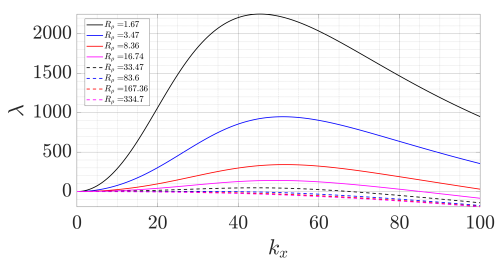
Figure 8. Growth rate as a function of density ratio and horizontal wavenumber for elevator mode \( {k_{z}} \) = 0 and square planform \( {k_{y}}={k_{y}} \) .

Table 4 shows the growth rate of the elevator mode with a square platform ( \( {k_{z}} \) = 0 249 and \( {k_{y}}={k_{x}} \) ) as a function of horizontal wavenumber \( {k_{x}} \) and the density ratio \( {R_{ρ}} \) . The growth rate presented in Figure 8 shows that the optimal wavenumber ( \( {k_{max}} \) ) is increasing while the density ratio is increasing. For the \( {R_{ρ}} \) value of 16.74 and 33.47, the results show that it crosses \( y \) -axis and reaches negative after \( {k_{max}} \) ≈ 50 − 70. The linear stability analysis does not predict any instability and associated finger width for the \( {R_{ρ}} \) > 100 based on the threshold value \( {R_{ρ}}=1/τ \) [10]. Nevertheless, the experiments also observe the formation of salt fingers with a density ratio \( {R_{ρ}} \) up to 334.7. The difference between the prediction of linear stability analysis and the experimentally measured finger width can be attributed to the following reason. The linear stability analysis assumes that the linear background temperature and salinity are maintained between the top and bottom boundaries. However, the experiments are more like run-down experiments because the temperature gradient and salinity gradient also vary slowly over time. As a result, here we only focus on case 4,5,6 with density ratio \( {R_{ρ}}∈ \) [8.36, 33.47] which is significantly smaller than 100 threshold value.

After obtaining the \( {k_{max}} \) that maximizes the growth rate of salt-finger instability, we then can obtain the corresponding wavelength as \( {λ_{max}}=2π/{k_{max}} \) . Then, we note that one wavelength corresponds to one upward and one downward plume, and thus the finger width \( {d_{LS}}={λ_{max}}/2=π/{k_{max}} \) . Then, we also convert this finger width to dimensional value that is \( {d_{LS*}}={d_{LS}}H=πH/{k_{max}} \) . Table 4 selected three values of \( {R_{ρ}} \) to analyse: 33.47, 268 16.74, and 8.36. This table shows the value of \( {k_{max}} \) , \( {d_{LS*}} \) predicted from linear stability and mean ( \( d \) ) from experimental measurements, which are in the same order of magnitude. Their difference may result from various reasons. For example, we have seen from the experimental results that individual fingers may merge into a wider finger, while the instability mechanism does not involve the interaction of many fingers.

6. Conclusion and future work

This work designs home-made experiments to investigate salt-finger convection which is an important process in ocean circulation. The experiment is done by pouring a designated concentration of salty hot water into the tank that contains a fixed amount of fresh, cold water. The temperature difference is fixed, and the concentration of salty water (salinity) is varied leading to different density ratios. A lower density ratio corresponds to a larger salinity difference between the top and bottom layer showing a stronger destabilizing effect. Salt fingers are visualized by dye and its displacement over time is obtained by recording using a camera and analysing video using Tracker.

These experiments effectively generate the phenomena resembling salt-finger microstructure in the ocean. The vertical and horizontal characteristic velocities of salt fingers are obtained from experiments over different density ratios. The vertical velocity is significantly increased by lowering the density ratio. Tilted fingers that resemble the experimental and oceanography observations are also observed and their trajectory is visualized. We also observe a non-zero horizontal velocity implying the presence of staircases. Finger widths over a range of density ratios obtained from the experiments are compared with that predicted from the linear stability analysis, which is within the same order of magnitude.

In future work, we can use apparatus with higher sensitivity, such as Particle Image Velocimetry (PIV) with a high-speed camera to obtain the velocity field of an entire region within the flow that can be detected simultaneously. This will significantly improve the current measurement technique which is based on point measurement methods with Tracker to analyse the spatio-temporal experimental data. The current analysis of salt-finger convection is mainly based on observing its movement from the side view (two-dimensional). Further analysing the measurement from the bottom view and reconstructing the three-dimensional flow field would provide additional insight into salt-finger convection. Also, the size of the finger may get larger due to finger merging, which may increase the error of the experimental measurement on tracking salt fingers. Collecting the movement of the fingers underwater using PIV has the potential to track the fingers more accurately by penetrating into the core of the fingers. Moreover, further analysing the origin of horizontal motion of salt fingers observed in these experiments through including the non-linear effect is also an interesting direction.

References

[1]. Turner, J. Double-diffusive phenomena. Annual Review of Fluid Mechanics 1974, 6, 37–56.
[2]. Schmitt, R.W.; Perkins, H.; Boyd, J.; Stalcup, M. C-SALT: An investigation of the thermohaline staircase in the western tropical North Atlantic. Deep Sea Res. Part A 1987, 34, 1655–1665.
[3]. Tait, R.; Howe, M. Thermohaline staircase. Nature 1971, 231, 178–179.
[4]. Padman, L.; Dillon, T.M. Thermal microstructure and internal waves in the Canada Basin diffusive staircase. Deep Sea Res. Part A 319 1989, 36, 531–542.
[5]. Schmitt, R.W. Double diffusion in oceanography. Annual Review of Fluid Mechanics 1994, 26, 255–285.
[6]. Shirtcliffe, T.; Turner, J. Observations of the cell structure of salt fingers. Journal of Fluid Mechanics 1970, 41, 707–719.
[7]. Yang, Y.; Verzicco, R.; Lohse, D. Scaling laws and flow structures of double diffusive convection in the finger regime. J. Fluid 323 Mech. 2016, 802, 667–689.
[8]. Stern, M.; et al. MAXIMUM BUOYANCY FLUX ACROSS A SALT FINGER INTERFACE. Journal of Marine Research 1976, 34, 95–110.
[9]. Stern, M.E. Collective instability of salt fingers. J. Fluid Mech. 1969, 35, 209–218.
[10]. Radko, T. Double-diffusive convection; Cambridge University Press, 2013.
[11]. Shen, C.Y. Heat-salt finger fluxes across a density interface. Physics of Fluids A: Fluid Dynamics 1993, 5, 2633–2643.
[12]. Schmitt, R.W.; Ledwell, J.; Montgomery, E.; Polzin, K.; Toole, J. Enhanced diapycnal mixing by salt fingers in the thermocline of the tropical Atlantic. Science 2005, 308, 685–688.
[13]. Tait, R.; Howe, M. Some observations of thermo-haline stratification in the deep ocean. Deep Sea Res. Oceanogr. Abstr. 1968, 15, 275–280.
[14]. Radko, T. A mechanism for layer formation in a double-diffusive fluid. J. Fluid Mech. 2003, 497, 365–380.
[15]. Radko, T. What determines the thickness of layers in a thermohaline staircase? J. Fluid Mech. 2005, 523, 79–98.
[16]. Radko, T. Equilibration of weakly nonlinear salt fingers. J. Fluid Mech. 2010, 645, 121–143.
[17]. Yang, Y.; Chen, W.; Verzicco, R.; Lohse, D. Multiple states and transport properties of double-diffusive convection turbulence. Proc. Natl. Acad. Sci. 2020, 117, 14676–14681.
[18]. Krishnamurti, R. Double-diffusive transport in laboratory thermohaline staircases. J. Fluid Mech. 2003, 483, 287–314.
[19]. Krishnamurti, R. Heat, salt and momentum transport in a laboratory thermohaline staircase. J. Fluid Mech. 2009, 638, 491–506.
[20]. Taylor, J.; Bucens, P. Laboratory experiments on the structure of salt fingers. Deep Sea Res. Part A 1989, 36, 1675–1704.
[21]. Roquet, F.; Madec, G.; Brodeau, L.; Nycander, J. Defining a simplified yet “realistic” equation of state for seawater. Journal of Physical Oceanography 2015, 45, 2564–2579.
Cite this article
Wang,S.;Liu,C. (2023). An experimental investigation on salt-finger convection. Theoretical and Natural Science,9,1-13.
Data availability
The datasets used and/or analyzed during the current study will be available from the authors upon reasonable request.
Disclaimer/Publisher's Note
The statements, opinions and data contained in all publications are solely those of the individual author(s) and contributor(s) and not of EWA Publishing and/or the editor(s). EWA Publishing and/or the editor(s) disclaim responsibility for any injury to people or property resulting from any ideas, methods, instructions or products referred to in the content.
About volume
Volume title: Proceedings of the 3rd International Conference on Computing Innovation and Applied Physics
© 2024 by the author(s). Licensee EWA Publishing, Oxford, UK. This article is an open access article distributed under the terms and
conditions of the Creative Commons Attribution (CC BY) license. Authors who
publish this series agree to the following terms:
1. Authors retain copyright and grant the series right of first publication with the work simultaneously licensed under a Creative Commons
Attribution License that allows others to share the work with an acknowledgment of the work's authorship and initial publication in this
series.
2. Authors are able to enter into separate, additional contractual arrangements for the non-exclusive distribution of the series's published
version of the work (e.g., post it to an institutional repository or publish it in a book), with an acknowledgment of its initial
publication in this series.
3. Authors are permitted and encouraged to post their work online (e.g., in institutional repositories or on their website) prior to and
during the submission process, as it can lead to productive exchanges, as well as earlier and greater citation of published work (See
Open access policy for details).