Calculating non-scalar diffraction efficiently via merging Braunbek method and Bluestein method

1. Introduction

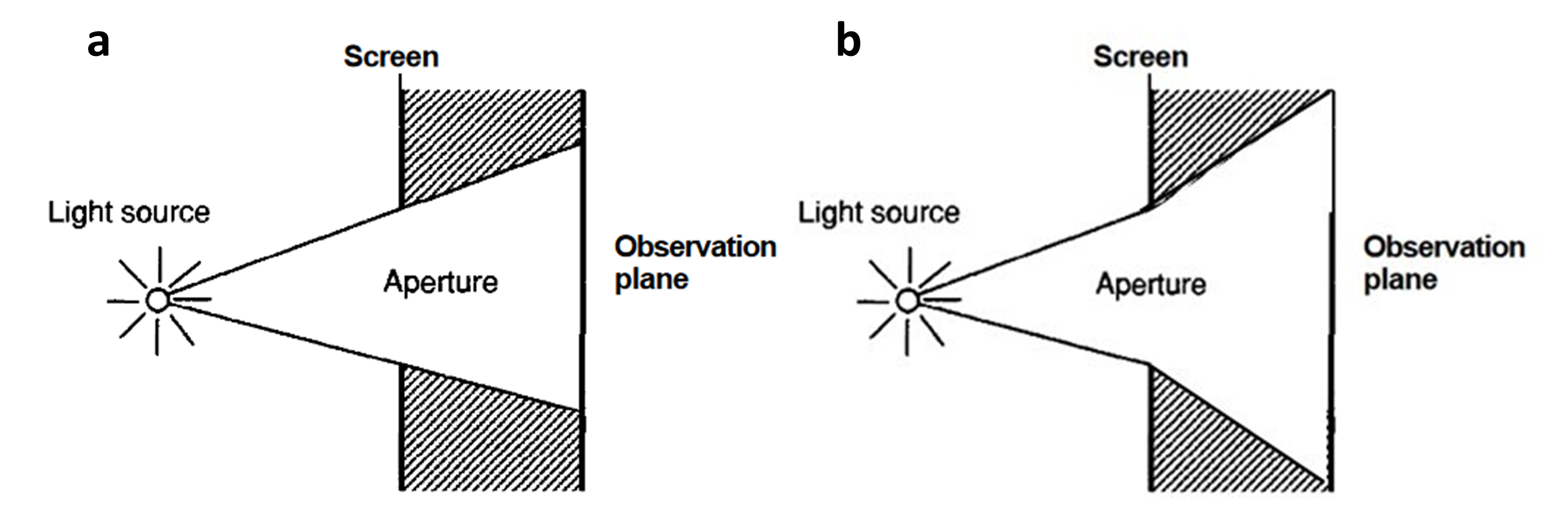
Diffraction is the bending of travelling light waves when they pass through obstacles or openings. The diffracted waves then interfere with each other to form new waves of various amplitudes. Apparent diffraction phenomena are typically observed when incident light waves meet a screen with a small aperture, forming diffracted light that interferes with each other at the observation/image plane, as shown in Fig. 1b. The phenomenon has sparked great interest as diffracted light displays bright and dark fringes extending far into the geometrical shadows of an observation plane behind the aperture [1], contradicting the geometrical optics theory shown in Fig 1a.

Figure 1. Arrangement for observing diffraction of light. a) Light field distribution predicted by geometrical optics theory. b) Actual light field distribution due to occurrence of diffraction [1]

The prediction of diffraction patterns is significant to many optical systems, including coronagraphs (large scale occulters (obstacles) that block portions of star light so as to better identify exoplanets), diffractive optical elements (DOE), and microscopy. In particular, extensive investigation into modelling diffraction from a starshade, a particular design of coronagraphs [2], are conducted to predict optical performances of the system [3-5]. Because the dimensions of such coronagraphs ( $\approx 30 \ m$ in diameter) limit experimentation for optical performances, accurate optical model validation becomes critical for advancing coronagraph technologies. Ever since Grimaldi's first report on the diffraction phenomena in 1665, many scientists have attempted to come up with a reasonable explanation for the issue. Disagreeing with Isaac Newton's particle theory of light, Thomas Young gave the first explanation of diffraction that stemmed from the wave theory of light. From such assumptions, Young assumed further that diffraction arises as a result of the interference of an incident wave and a diffracted wave diverging from the edges [6]. The latter idea was soon replaced by the Huygens-Fresnel principle [1], which claimed that each point on the wavefront of a wave can be considered a new source of a secondary spherical wave, and the wavefront at a later instant would be found by constructing the envelope of the secondary wavelets. From these principles, Kirchhoff constructed his theory of diffraction by solving the Helmholtz equation (derived from Maxwell's equation for electromagnetic waves) for a scalar component of amplitude (denoted by $\phi_s$ ) [1]. The derivation ultimately led to the famous Kirchhoff diffraction equation that matched remarkably well with experiments of the time. Furthermore, the equation was similar to that of a Fourier transform (FT), which shed light on subsequent research searching for efficient calculations of diffraction [7,8]. Even though Kirchhoff's diffraction theory became predominant for its surpassing accuracy, many simplifications and assumptions were made in its derivation. Some approximations have negligible impacts and are commonly adopted. Paraxial approximations are often still assumed, and dielectric mediums in which light propagates are still assumed to be linear, isotropic, homogeneous, and non-dispersive [1]. However, other assumptions are found to be inherently flawed, namely Kirchhoff's boundary conditions, which state [1]

Across the aperture, the field distribution and its normal derivative are exactly the same as they would be in the absence of the screen.
Over the portion of screen that lies in the geometrical shadow of the screen, the field distribution and its derivative are identically zero.

While these assumptions appear to be correct intuitively, they (a) encountered mathematical inconsistencies due to over-specification of boundaries and (b) ignored the effects of polarization. The first issue was that the assumptions implied a zero field all across the aperture and the screen due to the requirement that the field and its normal derivative must both be zero at the screen, which is obviously not the case for the actual diffraction phenomena. This issue was later resolved by replacing the Kirchhoff diffraction equation with the Rayleigh-Sommerfield diffraction equation [9], which accounted for either the absence of field or its normal derivative at the screens. The second issue is especially apparent in quasi-optical ranges where deviations in the vicinity of the aperture seam are fairly large [10]. It can be resolved through brute-force by direct calculation of Maxwell's equations for electromagnetic waves, but this method nullifies the efficiency. It appears, despite ongoing investigations, that there are still methods to calculate diffracted fields that lack both efficiency and accuracy. This paper proposes a more efficient and accurate method for calculating diffraction through insights from the Braunbek method [11] and the Bluestein method [12]. To recover boundary conditions, fields at the edges of the aperture are replaced with the exact fields calculated through Maxwell's equations. The rest of the fields at the aperture and screen are assigned Sommerfield's boundary values. Then, a chirp-Z-transformation (CZT) is utilised instead of standard Fourier optics techniques and fast Fourier transform techniques to improve efficiency and flexibility. The method reduces time complexity for computation and allows for arbitrarily chosen regions of interest and sampling numbers. The efficiency and accuracy of the method are exemplified through its comparison with existing models for predicting diffraction from rectangular aperture. The results are encouraging and show that the method is similar, if not superior, to existing models in terms of efficiency and accuracy in predicting diffraction patterns. Section 2 derives the mathematical model for this paper. Section 3 outlines the implementation of computational techniques. Section 4 presents our results along with those of previous methods. Section 5 compares different results and explains how our model achieves greater accuracy and efficiency. Section 6 restates the conclusions drawn from this work.

2. Model derivation

To predict the diffracted fields from a rectangular aperture, a mathematical model that recovers boundary conditions based on Sommerfield's solution is formulated in this section. The Braunbek method is implemented by replacing fields at the seam with exact fields to account for the non-scalar nature of electromagnetic waves. There are several key assumptions that have been kept in this paper. Outlined briefly in Section [???], they are

Paraxial approximations: the angle $\theta$ between light rays of the optical system and its reference axis remains small, such that $\theta \ll 1$ rad
Diffracted fields of interest are located in the near field, where the Fresnel number ( $F=a^2/L\lambda$ ; $$a$$ is aperture size; $$L$$ is distance from aperture; $\lambda$ is wavelength) satisfies the relation $F\theta^2/4 \ll 1$
Light propagates through dielectric mediums that are linear, isotropic, homogeneous, and non-dispersive
At regions apart from the edges of the seam, Sommerfield's boundary values are assigned at the screen and the aperture
The diffracted field $\phi$ satisfies Sommerfield's radiation condition at infinity [13]

2.1. Rayleigh-Sommerfield diffraction equation

2.1.1. Helmotz equation

The derivation of the Helmotz equation for electromagnetic waves stemmed from the most fundamental case of Maxwell's equations. For a medium that lacked free charges and currents, Maxwell's equations can be written as

\begin{align} \mathbf{\nabla}\times\mathbf{E} \&= -\mu\ \frac{
tial\mathbf{H}}{
tial t}\nonumber
\mathbf{\nabla}\times\mathbf{H} \&= \epsilon\ \frac{
tial\mathbf{E}}{
tial t}\nonumber
\mathbf{\nabla}\cdot \epsilon \mathbf{E} \&= 0\nonumber
\mathbf{\nabla}\cdot \mu \mathbf{H} \&= 0 \end{align}

where $\mathbf{E}$ is the electric field and $\mathbf{H}$ is the magnetic field. $\epsilon$ and $\mu$ are the electric permittivity and the magnetic permeability, respectively, of the medium through which light propagates.The media considered in this paper have vacuum magnetic permeability $\mu_0$ and constant electric permittivity $\epsilon$ . Combining these equations and making relevant simplifications [1], we obtain Helmotz equation for electromagnetic waves

\begin{equation} \nabla^2 \mathbf{E} - \frac{n^2}{c^2}\frac{
tial^2\mathbf{E}}{
tial t^2}=0 \end{equation}

where $$n$$ is the refractive index of the medium and $$c$$ is the speed of light. For the sake of simplicity, a scalar field $\phi_s$ mentioned in Section [???] is induced instead of $\mathbf{E}$ . Because all scalar components of $\mathbf{E}$ satisfies the same Helmotz equation, $\phi_s$ can be used to represent all scalar amplitudes. Hence, the scalar equation can be written as

\begin{equation} \nabla^2 \phi - \frac{n^2}{c^2}\frac{
tial^2\phi_s}{
tial t^2}=0 \end{equation}

The equation can be simplified further given an expression for $\phi$ . On that note, a complex function can be implemented to represent the transverse electromagnetic wave

\begin{equation} \tilde{\phi}_s(P, t) = \tilde{A}(P)e^{-i2\pi \nu t} \end{equation}

where $\tilde{A}(P)$ represents the complex amplitude of the wave that accounts of both amplitude and phase-shift, and $e^{-i2\pi \nu t}$ represents the oscillating term of the field as a given function of $$t$$ . Hence, substituting Eq. [???] into Eq. [???], a Helmotz equation of $\phi$ , a complex function of position only, is given to be

\begin{equation} \nabla^2 \phi + k^2 \phi = 0 \end{equation}

Here, $$k$$ is the wave number, given by $2\pi / \lambda$ ( $\lambda$ is the wavelength in the dielectric medium). Note that $\phi$ here only represents the complex amplitude of the wave, so it should not be confused with $\phi_s$ in Eq. [???] and Eq. [???].

2.1.2. Greens function

To solve for the field $\phi$ at a point $$P$$ , Greens theorem was used in part with Helmotz equation. The Green's theorem states,

Theorem: Let $\phi(P)$ and $$G(P)$$ be any two complex-valued functions of position, and let $$S$$ be a closed surface surrounding a volume $$V$$ , with normal $\mathbf{\hat{n}}$ . If $\phi$ , $$G$$ , and their first and second partial derivatives are single-valued and continuous within and on $$S$$ , then we have

\begin{equation} \iiint_{V}{( \phi\nabla^{2}G - G\nabla^{2}\phi )dV} = \iint_{S}{( \phi\frac{
tial G}{
tial n} - G\frac{
tial \phi}{
tial n} )dS} \end{equation}

Here, $\phi$ is apparently still the field potential at a point, while the auxiliary function $$G(P)$$ (also known as Greens function) are to be arbitrarily chosen such that a solution to $\phi$ can be obtained from it. The selection of Greens functions in this case are essential because various assumptions of the Greens function can lead to different solutions. Note that the choice of Greens functions are closely related to the boundary conditions of the solution. Formerly, Kirchhoff selected the Greens function to be an unit-amplitude spherical wave expanding about a point $$P_0$$ of interest. Its function of an arbitrary point in the region can be expressed as

\begin{equation} G_k(P)=\frac{e^{ikr_0}}{r_0} \end{equation}

where $$r_0$$ is the distance from $$P_0$$ to $$P$$ . However, since Kirchhoff's selection of Greens function are related to his assumptions on boundary conditions in Section [???], certain problems with his assumptions cannot be safely neglected. Specifically, Kirchhoff's boundary conditions required both the field and its normal derivative to be zero at the screen and aperture. This is impossible given that the solution is obviously non-zero in the plane of screen. Instead, Sommerfield's method assumed either field strength or its normal derivative to be zero. These conditions led to the first and second Rayleigh-Sommerfield Greens function, respectively. Only the first Greens function is selected in this paper for its simplicity [1].

2.1.3. First Rayleigh-Sommerfield solution

Assume that the new Greens function is composed of two expanding spherical waves. One expanding from the point of interest $$P_0$$ , while the other expands from a point $\tilde{P_0}$ that is a reflection of $$P_0$$ about the screen. Let vectors $\mathbf{r_0}$ and $\mathbf{\tilde{r_0}}$ represent the displacement from an arbitrary point $$P$$ to $$P_0$$ and $\tilde{P_0}$ , respectively. The normal $\hat{n}$ points orthogonal to the screen along the direction of $\mathbf{r_0}$ . The formalism is shown in Fig. 2.

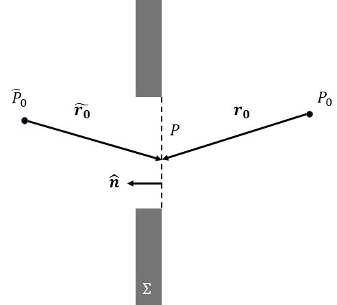
Figure 2. Geometry of first Rayleigh-Sommerfield Greens function.

To ensure that the field $\phi$ is zero across the aperture, a $\pi$ phase difference between the two sources $$P_0$$ and $\tilde{P_0}$ is assumed. Thus, the new Greens function is given by

\begin{equation} G(P)=\frac{e^{ikr_0}}{r_0}-\frac{e^{ik\tilde{r_0}}}{\tilde{r_0}} \end{equation}

Since the Greens function is expressed as the combination of two waves, it also satisfies the Helmotz equation for itself, that is

\begin{equation} \nabla^2 G + k^2 G = 0 \end{equation}

Returning to the diffraction problem, once Greens function was defined, a solution for $\phi$ could be obtained. Hence, defining an arbitrarily appropriate closed volume, Eq. [???] and [???] can be substituted in theorem [???] to give a solution to the the field $\phi$ (see Appendix A). In the case of an plane diffraction form an aperture, the solution is written in the form

\begin{align} \phi(P_0) \&= -\frac{1}{4\pi}\iint_\Sigma \phi\frac{
tial G}{
tial n}dS \nonumber
\&= -\frac{1}{2\pi}\iint_\Sigma \phi\frac{
tial}{
tial n}(\frac{e^{ikr_0}}{r_0} )dS \end{align}

where the field $\phi$ at a point $$P_0$$ is expressed as a multiplication of incident field $\phi$ and the normal derivative of the Greens function integrated over the entirety of the plane of the screen (including aperture) $\Sigma$ . This is known as the first Rayleigh-Sommerfield diffraction (RS1) equation. The benefit of this solution is that it is mathematically consistent with itself by providing identical solutions with Kirchhoff's diffraction equation to $\phi$ except at boundaries. The first Rayleigh-Sommerfield solution assumes only the absence of $\phi$ at the screen that is not the aperture, and does not require the same for the field's normal derivative $tial \phi /tial n$ .

2.2. Braunbek method

2.2.1. Braunbek integral

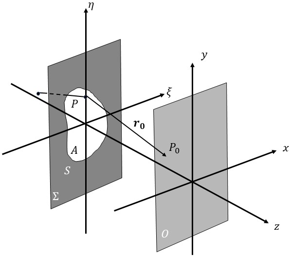
Based on the first Rayleigh-Sommerfield equation, Braunbek method provided modifications to further approach the exact solutions. The central idea of Braunbek method is to assume an additional wave diverging from the aperture edges. This contribution can arise from both the aperture side and the screen side of the edge. This idea was analogous to that of Thomas Young mentioned in Section [???], and it was in accordance to experiments [6]. Assume an incident plane wave travelling in the $$z$$ direction reaching an arbitrary aperture in the $\xi \eta$ -plane. The aperture is denoted $$A$$ , the screen is denoted $$S$$ , and their union is denoted $\Sigma$ . The observation plane ( $$xy$$ -plane) is denoted $$O$$ . As mentioned in Section [???], $$P$$ and $$P_0$$ represent an arbitrary point of disturbance on $\Sigma$ and an observed point on $$O$$ , respectively. The arrangement is shown in Fig. 3.

Figure 3. Coordinate system used in diffraction problem

Since the effects of a second wave is only apparent near edges, an RS1 integral that only counts the wave's contribution in the aperture side of the edge $$A'$$ and the screen side of the edge $$S'$$ was added. Hence, the combined RS1 solution was written as

\begin{equation} \phi(P_0) = -\frac{1}{2\pi}\iint_A \phi\frac{
tial}{
tial n}(\frac{e^{ikr_0}}{r_0})dS -\frac{1}{2\pi}\iint_{A'+S'} \phi\frac{
tial}{
tial n}(\frac{e^{ikr_0}}{r_0})dS \end{equation}

Notice that $$A$$ also contains $$A'$$ , so an superposition of waves was assumed in the overlapped region of $$A$$ and $$A'$$ . The second term on the right of Eq. [???] is known as the Braunbek integral $\phi_B$ , which assumes an additional wave in modification. Using the relation

\begin{equation} \frac{
tial }{
tial n}({\frac{e^{ikr_0}}{r_0}}) = (ik-\frac{1}{r_0})\frac{e^{ikr_0}}{r_0}\cos(\mathbf{n}, \mathbf{r}) \end{equation}

where $\cos(\mathbf{n}, \mathbf{r})$ is the cosine of the angle between vectors $\mathbf{\hat{n}}$ and $\mathbf{r_0}$ , the solution can be rewritten as

\begin{equation} \phi(P_0) = -\frac{1}{2\pi}\iint_A \phi (ik-\frac{1}{r_0})\frac{e^{ikr_0}}{r_0}\cos(\mathbf{n}, \mathbf{r_0})dS -\frac{1}{2\pi}\iint_{A'+S'} \phi(ik-\frac{1}{r_0})\frac{e^{ikr_0}}{r_0}\cos(\mathbf{n}, \mathbf{r_0})dS \end{equation}

Considering the assumptions made in section [???], the expression can be approximated as

\begin{align} \phi(P_0) \approx \&-\frac{i}{\lambda}\iint_A \phi \frac{e^{ikr_0}}{r_0}\cos(\mathbf{n}, \mathbf{r_0})dS \nonumber -\frac{i}{\lambda}\iint_{A'+S'} \phi \frac{e^{ikr_0}}{r_0}\cos(\mathbf{n}, \mathbf{r_0})dS \nonumber
\approx \& \ \ \frac{z}{i\lambda}\iint_A \phi \frac{e^{ikr_0}}{{r_0}^2} \ d\xi d\eta +\frac{z}{i\lambda}\iint_{A'+S'} \phi \frac{e^{ikr_0}}{{r_0}^2}\ d \xi d \eta \end{align}

Furthermore, the Fresnel approximation can be made on $$r_0$$ , that is,

\begin{align} r_0 \&= \sqrt{(x-\xi)^2+(y-\eta)^2+z^2} \nonumber
[5pt] \&= z\sqrt{1+(\frac{x-\xi}{z})^2+(\frac{y-\eta}{z})^2} \nonumber
[6pt] \&\approx z[1+\frac{1}{2}(\frac{x-\xi}{z})^2+\frac{1}{2}(\frac{y-\eta}{z})^2] \end{align}

where $$P$$ has coordinates $(\xi, \eta, 0)$ and $$P_0$$ has coordinates $$(x, y, z)$$ . Using the Fresnel approximation, along with some basic algebraic manipulations, the diffraction equation becomes

\begin{multline} \phi(P_0) \approx \frac{e^{ikz}}{iz\lambda}e^{\frac{ik}{2z}(x^2+y^2)}\Bigr[ \iint_A\phi(P)e^{\frac{ik}{2z}(\xi^2+\eta^2)} \times e^{-\frac{ik}{2z}(x\xi + y\eta)} \ d\xi d\eta
+ \iint_{A'+S'}\phi(P)e^{\frac{ik}{2z}(\xi^2+\eta^2)} \times e^{-\frac{ik}{2z}(x\xi + y\eta)} \ d\xi d\eta \ \Bigr] \end{multline}

Equation [???] is a generalized form of the modified diffraction equation. It is written in this form for convenient calculations, as the field at $$P_0$$ is basically the Fourier transform of the product of the optical disturbance $\phi(P)$ with a quadratic phase factor. This fact is exploited for computation in Section [???].

2.2.2. Polarization

The implementation of RS1 solution in Section [???] requires a known diffracted field distribution $\phi(P)$ immediately behind the aperture. Traditionally, the field is assumed to be unperturbed within the aperture so that $\phi(P)=\phi_0(P)$ , where $\phi_0 (P)$ is a scalar incident field. However, non-negligible perturbation of electromagnetic waves from edges of apertures have been shown more recently [5]. It was found that screens affect electric fields in a polarization-dependent manner. Hence, an estimation to $\phi(P)$ will be modified according to polarization of non-scalar fields. For convenience, the calculations for polarization are done in the normal coordinates of the edge shown in Figure 4. The unit vector $\mathbf{\hat{t}}$ is directed tangentially to the edge, the unit vector $\mathbf{\hat{n}}$ is directed normally to the edge, and the two are within the plane $\Sigma$ . Note that the normal referred to in Fig. 2 is not identical with that referred to in Fig. 4. The former indicates the normal to the plane of aperture, while the latter indicates the normal to the edge. The unit vector $\mathbf{\hat{z}}$ is orthogonal to both vectors and $\Sigma$ .

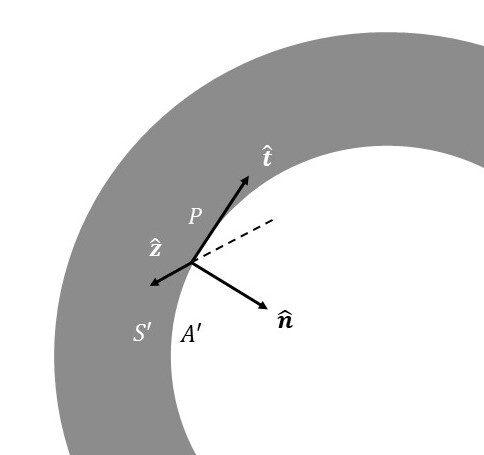
Figure 4. Edge coordinate system used in polarization orientation.

In addition, the field can be considered a linear combination of two orthogonal polarization states $$s$$ and $$p$$ , where each is directed in the $\mathbf{\hat{t}}$ and $\mathbf{\hat{n}}$ direction, respectively. Hence, the derivation for two simpler models suffice in explaining more complex models. By only considering the edges locally, the expressions for electric and magnetic field components are given by

\begin{equation} \mathbf{E} = (\phi, 0, 0), \ \ \ ik\mathbf{H}=(0, \frac{
tial \phi}{
tial z}, -\frac{
tial \phi}{
tial n}) \end{equation}

if incident field is s-polarized, and

\begin{equation} \mathbf{H} = (\phi, 0, 0), \ \ \ -ik\mathbf{E}=(0, \frac{
tial \phi}{
tial z}, -\frac{
tial \phi}{
tial n}) \end{equation}

if the incident field is p-polarized. Hence, the Braunbek integral can be rewritten in terms of s and p polarization states:

\begin{equation} \phi_{B,s} = \frac{e^{ikz}}{iz\lambda}e^{\frac{ik}{2z}(x^2+y^2)}\iint_{A'+S'}E_t \ e^{\frac{ik}{2z}(\xi^2+\eta^2)} \times e^{-\frac{ik}{2z}(x\xi + y\eta)} \ d\xi d\eta \end{equation}

\begin{equation} \phi_{B,p} = \frac{e^{ikz}}{iz\lambda}e^{\frac{ik}{2z}(x^2+y^2)}\iint_{A'+S'}H_t \ e^{\frac{ik}{2z}(\xi^2+\eta^2)} \times e^{-\frac{ik}{2z}(x\xi + y\eta)} \ d\xi d\eta \end{equation}

where $$E_t$$ and $$H_t$$ are the electric and magnetic fields in the tangential direction. These equations were substituted into Eq. [???] to account for polarization at edges. For the actual evaluation of the exact vector fields, Finite-Difference Time-Domain (FDTD) methods are carried out by solving Maxwell's equation.

3. Computational implementation

3.1. Fourier Transform

In the theory of Fourier optics, diffraction could be understood as a transformation from incident field to a diffracted field by an obstacle. As demonstrated in [???], such transformation turns out to be the Fourier transform. Hence, Fourier analysis was adopted to reduce the difficulty of calculations. In optics, the 2D Fourier transform involves transforming functions from the space domain to the frequency domain, while the inverse Fourier transform transforms does vice versa. The transform is defined as

\begin{equation} \begin{split} \mathcal{F}\{ g(x,y) \} \&= \iint_{-\infty}^{\infty}g(x, y) e^{-i2\pi (f_x x + f_y y)}dxdy
\&= G(f_x, f_y) \end{split} \end{equation}

where $$g(x, y)$$ is a function in the space domain, and the Fourier transform transforms it into a function $$G(f_x, f_y)$$ in the frequency domain. Its reverse is defined as

\begin{equation} \begin{split} \mathcal{F}^{-1}\{ G(f_x, f_y)\} \&= \iint_{-\infty}^{\infty}G(f_x, f_y)e^{i2\pi(f_xx+f_yy)}df_xdf_y
\&= g(x, y) \end{split} \end{equation}

Returning to the diffraction equation, the Fourier transform identity can greatly reduce the complexity of Eqs. [???], [???], [???] in a simpler form, that is

\begin{equation} \phi(P_0) \approx \frac{e^{ikz}}{iz\lambda}e^{\frac{ik}{2z}(x^2+y^2)} \ \mathcal{F} \{ \phi(P)e^{\frac{ik}{2z}(\xi^2+\eta^2)} \} + \phi_B \ \end{equation}

where

\begin{equation} \phi_{B,s} = \frac{e^{ikz}}{iz\lambda}e^{\frac{ik}{2z}(x^2+y^2)}\mathcal{F} \{ E_t \ e^{\frac{ik}{2z}(\xi^2+\eta^2)} \} \end{equation}

\begin{equation} \phi_{B,p} = \frac{e^{ikz}}{iz\lambda}e^{\frac{ik}{2z}(x^2+y^2)}\mathcal{F} \{ H_t \ e^{\frac{ik}{2z}(\xi^2+\eta^2)} \} \end{equation}

Equation [???] can then be computed efficiently via numerical Fourier transform techniques. Traditionally, 2D Fast Fourier Transform (FFT) were implemented to calculate the expression in discrete form, where one value is sampled every sampling interval. Reducing the sampling number to minimum through the Nyquist-Shannon sampling theorem, the transformed function can be expressed as a set of discrete data with similar accuracy to analytical methods. The benefit of the FFT is that it only need $$O(n^2logn)$$ operations to transform a $n\times n$ grid. Till now, it is still a predominant method to calculating optical patterns due to its significant advantage compared to direct integration and standard FT. However, there are still minor deficiencies to the method which could be further modified, such as inflexible sampling resolutions.

3.2. Bluestein method

Even though the FFT is quite sufficient, it is restricted by the requirement that the number of discrete samples in the output plane must be equal to that in the input plane. For instance, if a large number of sampling numbers are required in the output plane for high resolution, the input plane must require the same number of samples either by increased resolution or zero-padding methods. This greatly reduces the efficiency by spending time on operating on zeros of the input. The Bluestein method is introduced to offer high-resolution outputs at arbitrary frequencies with arbitrary bandwidths. This is allowed by performing a Chirp-z transform along spiral contours in the z-plane for an input. Its transform is somewhat similar to the FFT, but a complex coefficient $$z$$ is used instead of the traditional coefficient. The formula is given by

\begin{equation} X[m]=\sum_{n=0}^{N-1}x[n]\times z^{-n} \Biggr|_{z=A\times W^{-m}} = \sum_{n=0}^{N-1}x[n]\times A^{-n}\times W^{mn} \end{equation}

where $$m = [0,...,M-1]$$ . $$M$$ is the length of the transform. $$N$$ is the length of input sequence. $$A$$ specifies the complex starting point of the z-plane spiral contour of interest, and $$W$$ is a complex scalar describing the complex ratio between neighboring points on the contour.By their definition, $$A$$ and $$W$$ can be expressed as

\begin{equation} A = A_0 e^{i\theta_0} \end{equation}

and

\begin{equation} W = W_0 e^{i\phi_0} \end{equation}

where $$A_0$$ and $\theta_0$ indicates the radius and angle of the complex starting point, respectively. $$W_0$$ and $\phi_0$ is the radius variance ratio of the spiral contour and the angular spacing between adjacent samples, respectively. Note that these parameters are applied to a unit circle in the z-plane which represents the frequency spectrum. An illustration of the unit circle for the FFT method and the CZT method is shown in Fig. 5. This method provides a generalized setup of the standard FFT, where more parameters could be freely chosen. It allows the selection of arbitrary starting points and ending points for frequency, arbitrary sampling numbers, and arbitrary length of samples. On the other hand, the standard FFT specifies the parameters to be $$A_0=1$$ , $\theta_0 = 0$ , $$W_0=1$$ , $\phi_0 = -2\pi /N$ , and $$M=N$$ . For this paper, the parameters are chosen to be

\begin{equation} A = - e^{i2\pi f_1/f_s} \end{equation}

\begin{equation} W = e^{-i2\pi (f_2-f_1)/Mf_s} \end{equation}

where $$f_1$$ is the starting point along the sampled contour, $$f_2$$ is the ending point, and $$f_s$$ is the dimension of the output plane along both vertical and horizontal direction. A comparison of the approach with that of the traditional

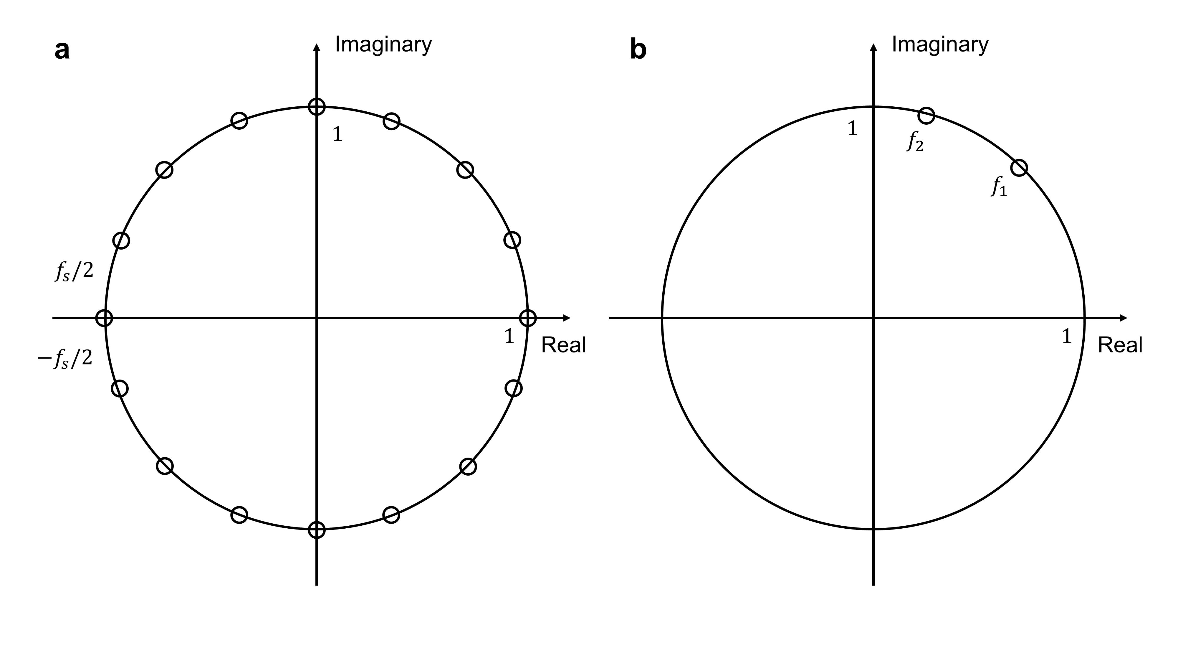
Figure 5. Comparison of the FFT and the CZT on the z-plane

FFT is shown in Fig. 5. While the FFT in Fig. 5a samples at a constant sampling frequency along the unit circle (which represents the full frequency spectrum), the approach adopted in this paper only samples along a region of interest of the unit circle. This allows a reduction in sampling frequency, which enables sampling a signal in fewer samples. Moreover, the starting point, ending point, region of interest, and the size of the output plane can all be arbitrarily chosen. Note that this approach is only one possible way in computing the FT. Due to the flexibility of the CZT, and part of the z-plane can be sampled, including regions that are not on the unit circle. The Bluestein method is implemented to compute Eq. [???] in Matlab [14]. A variation of the CZT or Bluetein method in the context of Fourier optics is developed by [8] and applied in this paper.

3.3. Simulation

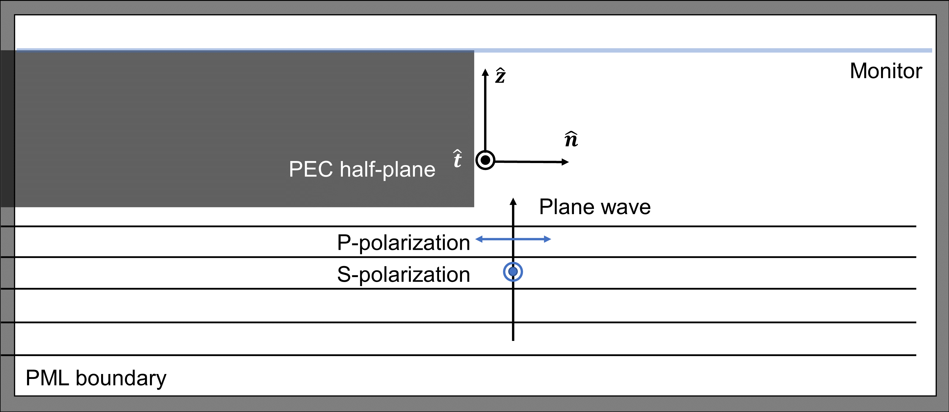
As mentioned Section [???], the exact fields at the edges of the aperture are to be numerically calculated by FDTD methods. The method was implemented through a built-in FDTD solution software by Lumerical [15]. A plane wave source of s- and p-polarization was each designed to pass a infinite half-plane, and the field distribution immediately behind the edge was monitored. The light waves simulated had wavelength $\lambda = 600 \ nm$ . The thickness of the half-plane was $10 \ nm$ , and it was designed to be perfectly electric conductive (PEC) material. Perfectly matched layers (PML) were created at boundaries to simulate open-boundaries. The setup is illustrated in Fig. 6. After the simulation, recorded electric fields and magnetic fields were substituted in Eqs. [???] and [???] as functions of location.

4. Results

4.1. Polarization

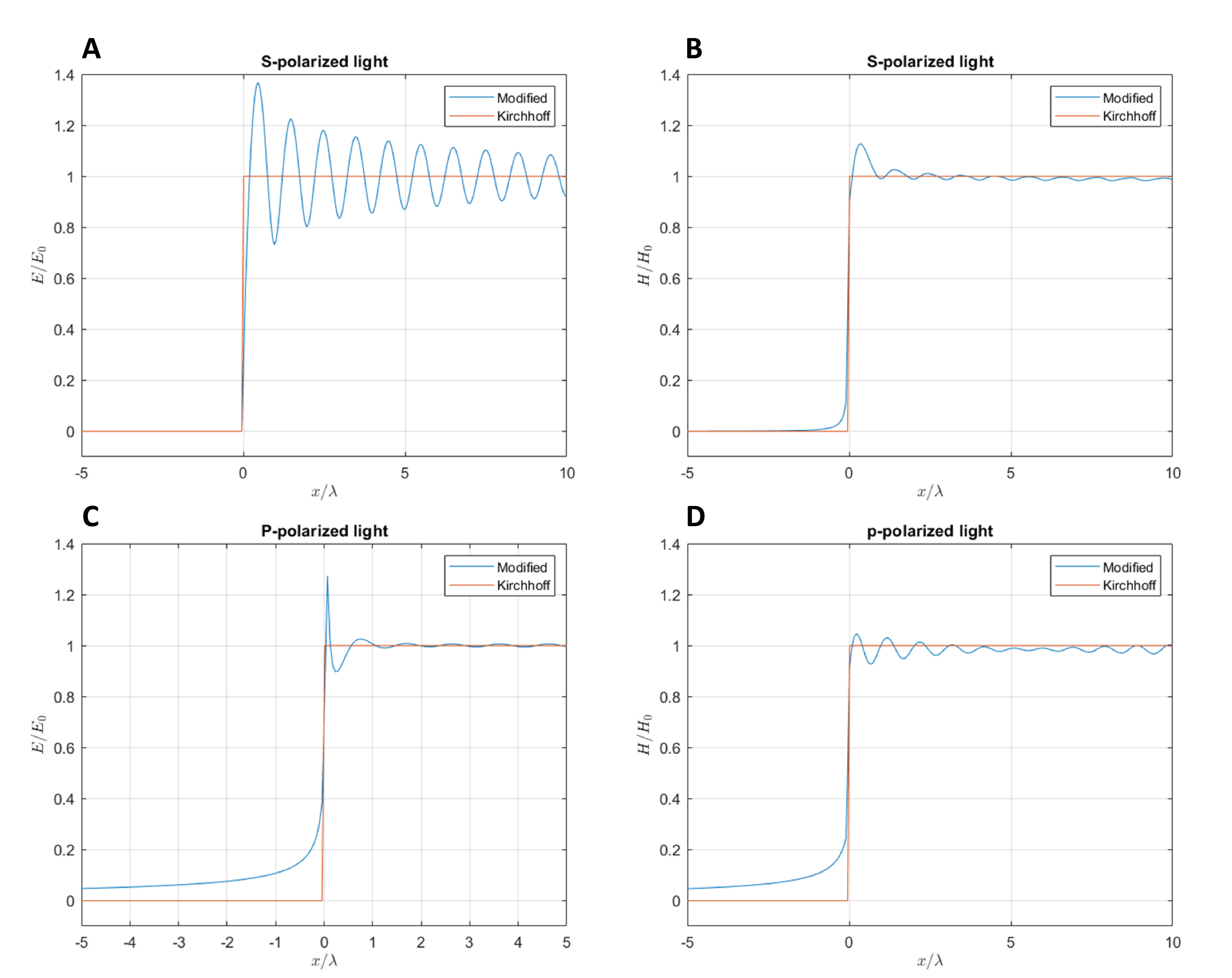
For both s- and p-polarizations, the exact values of the electric and magnetic fields are evaluated (in the vicinity of a straight edge and immediately behind the aperture) in Fig. 6. Here, the x-axis indicates the distance from the edge in terms of wavelengths. The y-axis indicates the ratio between the field immediately behind the aperture and that of incidence. The red line indicates Kirchhoff's predicted field according to his assumptions in Section [???]. The blue line indicates the simulated exact fields. The electric field for s-polarized light shows the greatest deviation from Kirchhoff's assumed field. Its oscillation peaks to $\approx 1.4$ and then gradually tends to 1. The fields from 7b, 7c, 7d are all approximately in accordance with Kirchhoff's assumed field. However, there are still visible oscillations around the discontinuity at $$x=0$$ . The electric and magnetic fields of p-polarized light were both non-zero within the screen ( $x\lt 0$ ), while those of s-polarized light were close to zero.

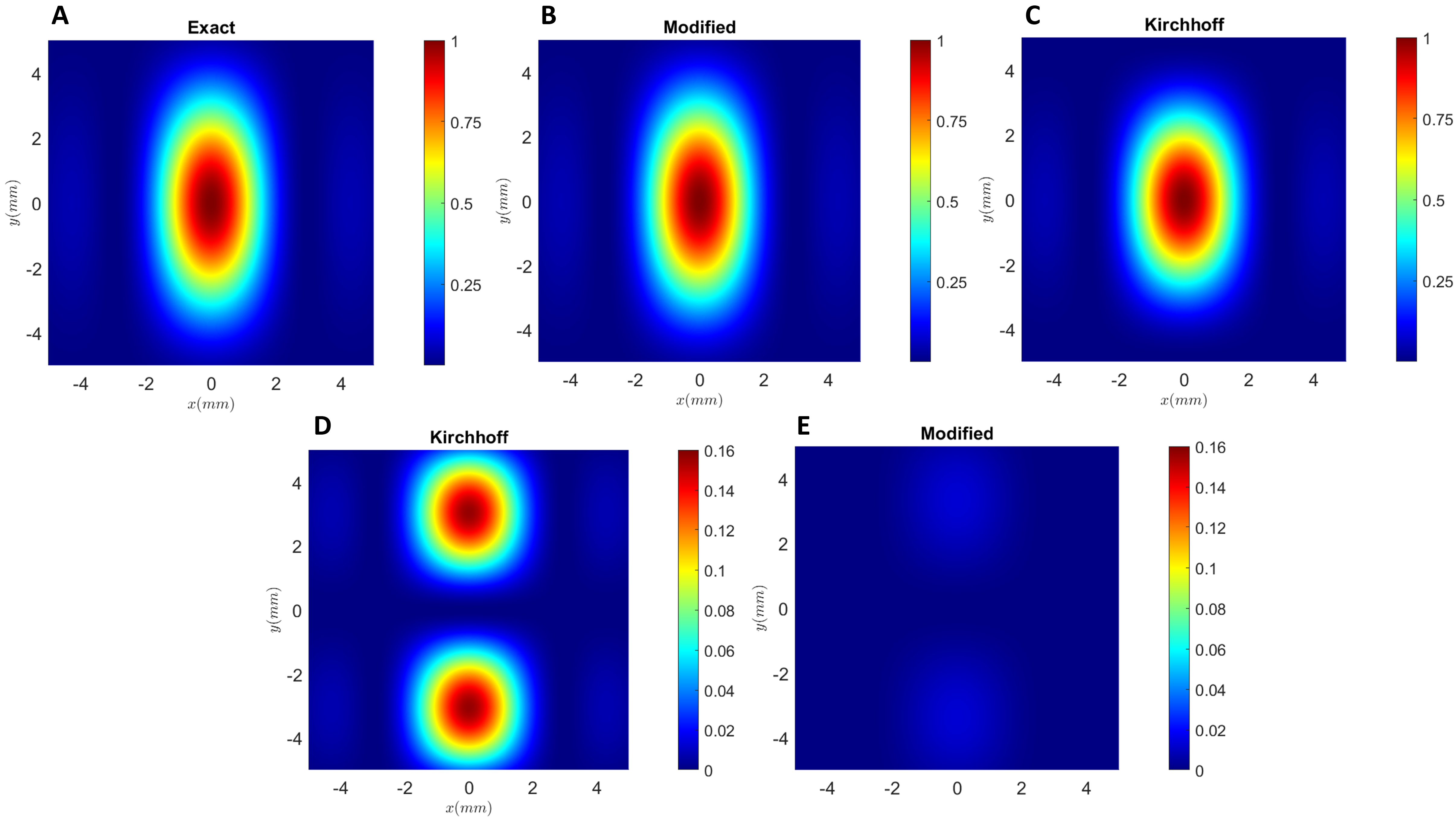
Figure 7. Evaluation of exact fields around straight edge. All values evaluated in this figure refers to the component corresponding to its polarization. a) Electric field for s-polarization b) Magnetic field for s-polarization c) Electric field for p-polarization d) Magnetic field for p-polarization. Results of simulation from Lumerical [15]

4.2. Diffraction pattern

Fig. 8 presents the light intensity of three different diffraction patterns, each from a different solution. The configuration is designed with a $12 \ \mu m \times 6 \ \mu m$ rectangular aperture and a $5 \ mm \times 5 \ mm$ observation plane (region of interest) located $60 \ mm$ from the screen. The resolution of both the input plane and the output plane is designed to be $1080 \times 1080$ grids. A plane wave light source with a wavelength $600 \ nm$ and s-polarization is assumed. The distribution of light intensity, a term (denoted $$I$$ ) proportional to $\phi^2$ , is shown with respect to location, and the color bar indicates the ration between $$I$$ and the intensity $$I_0$$ of the incident light from $$0$$ to $$1$$ . Fig. 8a, the exact field distribution, is obtained by simulating the diffracted fields with exact values at boundaries retrieved using FDTD methods. On the other hand, Fig. 8b and Fig. 8c, were calculated by implementing modified boundary conditions and Kirchhoff's assumed boundaries, respectively. The shapes of all three figures are similar, forming concentric oval rings at the centre and first-order bright and dark fringes at the sides. However, Fig. 8a and 8b appear to have a longer major axis of their elliptical ring than Fig. 8c do. The field distribution difference between each of the solution (kirchoff and modified braunbek solution) and the exact solution is presented in figure 8. A more apparent comparison can be made seeing that there is a larger difference between the exact solution and the kirchoff solution primarily emerging from the two tips of the oval in the diffraction pattern. On the other hand, a much smaller difference is seen between the exact solution and the modified solution.

Figure 8. Diffraction pattern of light through rectangular slits computed through a) Exact solution b) Modified solution c) Kirchhoff solution. d) Light distribution difference between the exact solution and the Kirchhoff solution. e) Light distribution difference between the exact solution and the modified solution. Diffraction patterns are generated in Matlab [14].

Figure 9. Comparison of computation time between FFT and CZT. Recorded using Matlab [14].

4.3. Computation time

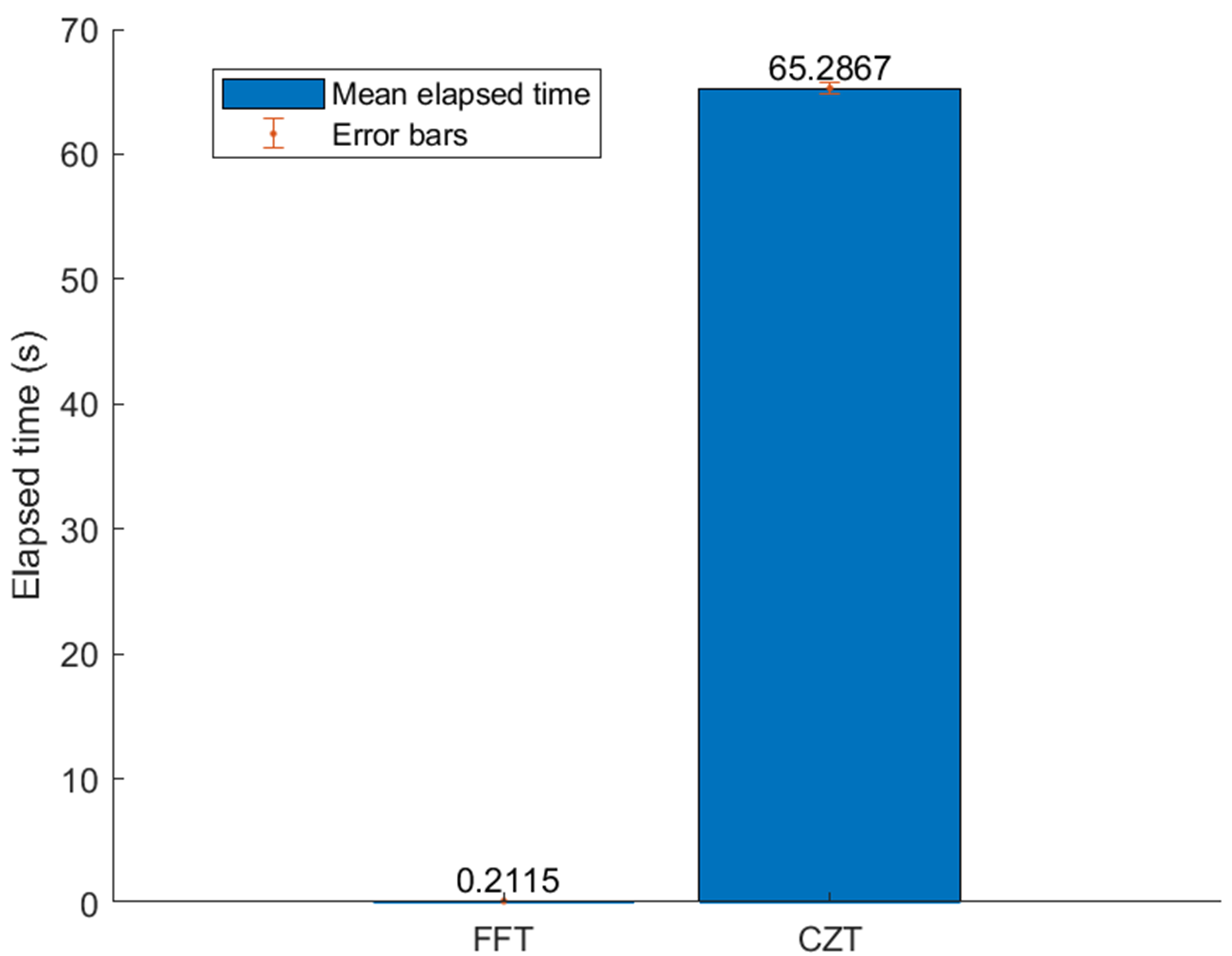
The elapsed time for FFT and CZT were recorded for the calculation of the modified diffraction pattern. The FFT method required a time of 62.1 seconds while the CZT method required a time of 0.184 seconds. The time for direct integration method were not recorded because of its immense calculation that is not supported by the device.

5. Discussion

5.1. Polarization

In order to predict diffraction with accuracy, a modified boundary condition was retrieved using FDTD methods outlined in [???]. The modified field distribution is mostly in accordance to both theory [10] and experimentation [5]. It was previously conjectured that the tangential component of the electric field vanishes at the edge while the perpendicular component approaches infinity. The former corresponds to the sharp decrease at $$x=0$$ in Fig. 7a while the latter corresponds to the sharp peak at $$x=0$$ in Fig. 7c (the peak in the figure only reaches up to $\approx 1.3$ because of the restriction that the graph is plotted with discrete values). However, recorded data was less in accordance with theory for magnetic fields. It was conjectured that the tangential component of the magnetic field remains finite at edges while the perpendicular component approaches infinity. Apparently, Fig. 7d matches the former, but Fig. 7b fails to match the latter case. This is possibly due to the variability in magnetic permeability, a failure in simulation process at discontinuities, or other reasons that may be further investigated. Another confirmation for Fig. 7a is Harness[5]. Fig. 7a matched closely with both Sommerfield's half-plane solution and simulation results for $7 \ \mu m$ Si $$+$$

$0.4 \ \mu m$ Au material screen. The results obtained in Fig. 8 are expected to be applicable to most conductive materials with similar width, and it can be of great importance to the understanding of field perturbation at edges of materials.

5.2. Diffraction pattern

Figure 8 shows an improved model to predict diffraction patterns that matches more closely to the actual diffraction patterns. Both models have generated a similar pattern: elliptical bright spot in the centre arising from the majority of light from the aperture. The bright and dark fringes appear consecutively due to constructive and destructive interference, respectively. However, there are some key differences in terms of the shape of each solution. The bright ellipse in the centre of the diffraction pattern stretches longer than that of Kirchhoff's prediction. This is due to the account for an additional light source at the edges discussed in Section [???], Section [???], and Rubinowicz [6]. This is especially apparent when looking at the differences between each solution's field distribution with that of the exact solution, where two additional bright spots coming from the edge is obviously discounted by Kirchhoff's solution. There is a much larger deviation in the Kirchhoff's estimation along the width rather than the length of the hypothetical rectangular aperture because the effects of polarization and neglected edge effects are only apparent within a few wavelengths at apertures that are especially comparable to its size. A similar but much smaller difference (approximately ten times smaller difference) is observed in the difference of the modified and exact solution fields. This is due to the degree of approximations taken while deriving the Braunbek equations. The results were in accordance with Harness [5], in which they also demonstrated how the modified results matched closer to the experimental results that the Kirchhoff and Sommerfield solutions did. However, in their work, there is a much more significant difference (an order of magnitude difference) between the modified solution and the previous solutions. Such significant differences are suspected to arise from the dimensions ( $35 \ mm$ diameter occulter and $80 \ m$ long testbed) that Harness [5] worked with and the complex shape of the star-shade. The differences shown in Fig. 8 are expected to become less apparent as the size of the aperture increases because the modification only acts on the local edges of the aperture. Nevertheless, the results from Fig. 8 successfully proven the superior accuracy of the model in this paper, and its application can be particularly significant to the fields of small-scale optical instruments.

5.3. Computation time

One of the main goals of this paper was to develop a more efficient method to calculate diffraction patterns. Fig. 9 shows that our method successfully exceeds the traditional FFT by $\approx 1 \ min$ . The vast difference in calculation times lies in the inflexibility of the FFT. In order to extend the output region of interest, the FFT requires a huge number of padding operations. In this case, by almost three orders of magnitude. On the other hand, the CZT eliminates all those operations using a spectral zoom operation with high resolution and arbitrary bandwidth. The results were in close accordance with those presented by Hu[8]. The time of computation was increased by $\approx 6 \ s$ and $0.5 \ s$ for FFT and CZT in their study, respectively. This is due to the reduction in the complexity and dimensions of our scenario. The distance between the observation plane and screen is reduced by an order of magnitude, the dimension of the aperture is reduced by about three orders of magnitude, and the aperture is simplified from a convex lens to a rectangular slit. Fig. 9 confirms the validity of our method for fast calculation of diffractive fields, and such methods can be widely implemented for not only optical systems that require a flexible region of interest and resolution but also for other fields such as image processing that require a more flexible FT method.

6. Conclusion

This paper investigates the calculation of non-scalar diffraction with efficiency and accuracy through the implementation of the Braunbek and Bluestein methods. First, a mathematical model was derived to modify Kirchhoff's assumed boundary conditions and address the non-scalar component of electromagnetic waves. Next, the CZT is implemented to compute the FT identified in the derivation with more flexibility, allowing arbitrary regions of interest, sampling points, frequency, and resolution. Finally, the simulation results of electric and magnetic fields at boundaries are presented and the calculated diffraction pattern for various models is compared. The results demonstrated mostly good agreement with other literature. The Braunbek method modifies Kirchhoff's assumptions on boundaries and enhances the accuracy of predicting diffraction patterns for small apertures. The Bluestein method quickens the process by implementing the CZT in a way that allows for a much more flexible range and resolution of computation. For optical systems such as coronagraphs with dynamic scales, the method developed in this paper is especially helpful because it eliminates the need for integrating point-by-point while still ensuring good accuracy. Apart from optical systems, the method discussed in this paper can also provide insight into enhancements in image processing and other realms that involve the FT. However, some limitations in this paper include the unmatched results between theoretical values and simulated values for the tangential component of the magnetic field; the lack of examination of our method for larger or smaller dimensions; and a comparison of more methods for calculating the FT. Furthermore, this paper still makes many assumptions for the sake of simplicity. The validation of the method still requires testing in closer proximity to more dynamic materials and more complex shapes.

References

[1]. Goodman J W 2005 Introduction to Fourier Optics (Roberts and Company Publishers) ISBN 0-9747077-2-4 978-0- 9747077-2-3

[2]. Cash W 2006 Nature 442 51–53 ISSN 1476-4687 number: 7098 Publisher: Nature Publishing Group URL https: //www.nature.com/articles/nature04930

[3]. Cash W 2011 The Astrophysical Journal 738 76 ISSN 0004-637X publisher: American Astronomical Society URL https://doi.org/10.1088/0004-637x/738/1/76

[4]. Harness A, Shaklan S, Cash W and Dumont P 2018 JOSA A 35 275–285 ISSN 1520-8532 publisher: Optica Publishing Group URL https://opg.optica.org/josaa/abstract.cfm?uri=josaa-35-2-275

[5]. Harness A 2020 Optics Express 28 34290–34308 ISSN 1094-4087 publisher: Optica Publishing Group URL https: //opg.optica.org/oe/abstract.cfm?uri=oe-28-23-34290

[6]. Rubinowicz A 1957 Nature 180 160–162 ISSN 1476-4687 number: 4578 Publisher: Nature Publishing Group URL https://www.nature.com/articles/180160a0

[7]. Barnett A H 2020 Efficient high-order accurate Fresnel diffraction via areal quadrature and the nonuniform FFT Tech. Rep. arXiv:2010.05978 arXiv arXiv:2010.05978 [astro-ph, physics:physics] type: article URL http://arxiv. org/abs/2010.05978

[8]. Hu Y, Wang Z, Wang X, Ji S, Zhang C, Li J, Zhu W, Wu D and Chu J 2020 Light: Science & Applications 9 119 ISSN 2047-7538 number: 1 Publisher: Nature Publishing Group URL https://www.nature.com/articles/ s41377-020-00362-z

[9]. Wolf E and Marchand E W 1964 JOSA 54 587–594 publisher: Optica Publishing Group URL https://opg.optica. org/josa/abstract.cfm?uri=josa-54-5-587

[10]. Bouwkamp C 1954 Reports on Progress in Physics 17 35–100 ISSN 0034-4885

[11]. Werner B 1949 URL https://link.springer.com/article/10.1007/BF01329835

[12]. Bluestein L 1970 IEEE Transactions on Audio and Electroacoustics 18 451–455 ISSN 1558-2582 conference Name: IEEE Transactions on Audio and Electroacoustics

[13]. Atkinson F 1949 The London, Edinburgh, and Dublin Philosophical Magazine and Journal of Science 40 645–651 ISSN 1941-5982 publisher: Taylor & Francis _eprint: https://doi.org/10.1080/14786444908561291 URL https: //doi.org/10.1080/14786444908561291

[14]. Matlab URL https://www.mathworks.com/products/matlab.html

[15]. Lumerical FDTD solution URL https://www.lumerical.com/

Cite this article

Yang,T.Z. (2023). Calculating non-scalar diffraction efficiently via merging Braunbek method and Bluestein method. Theoretical and Natural Science,9,132-150.

Data availability

The datasets used and/or analyzed during the current study will be available from the authors upon reasonable request.

Disclaimer/Publisher's Note

The statements, opinions and data contained in all publications are solely those of the individual author(s) and contributor(s) and not of EWA Publishing and/or the editor(s). EWA Publishing and/or the editor(s) disclaim responsibility for any injury to people or property resulting from any ideas, methods, instructions or products referred to in the content.

About volume

Volume title: Proceedings of the 3rd International Conference on Computing Innovation and Applied Physics

ISBN：978-1-83558-129-2(Print) / 978-1-83558-130-8(Online)

Editor：Yazeed Ghadi

Conference website: https://www.confciap.org/

Conference date: 27 January 2024

Series: Theoretical and Natural Science

Volume number: Vol.9

ISSN：2753-8818(Print) / 2753-8826(Online)

© 2024 by the author(s). Licensee EWA Publishing, Oxford, UK. This article is an open access article distributed under the terms and conditions of the Creative Commons Attribution (CC BY) license. Authors who publish this series agree to the following terms:
1. Authors retain copyright and grant the series right of first publication with the work simultaneously licensed under a Creative Commons Attribution License that allows others to share the work with an acknowledgment of the work's authorship and initial publication in this series.
2. Authors are able to enter into separate, additional contractual arrangements for the non-exclusive distribution of the series's published version of the work (e.g., post it to an institutional repository or publish it in a book), with an acknowledgment of its initial publication in this series.
3. Authors are permitted and encouraged to post their work online (e.g., in institutional repositories or on their website) prior to and during the submission process, as it can lead to productive exchanges, as well as earlier and greater citation of published work (See Open access policy for details).