1. Introduction

With China’s population rise, many people are jammed in most recreational places. People cannot have a good experience due to traffic jams, long queues, and crowding. Under the circumstances, preparing and designing a detailed plan that records the best route is necessary. For example, we choose a typical metropolitan city-shanghai and Disneyland, to be our fun places.

When people visit Disneyland in Shanghai, they may be annoyed since they must line up for the recreation facilities, which limit the items available each time, reducing satisfaction. Therefore, effectively arranging the waiting time and walking routes is essential to maximize visitors’ satisfaction. On the other hand, this research paper focuses on the waiting line problems and the dominant time cost in Shanghai Disneyland to offer visitors an enjoyable experience.

In this paper, 13 recreation facilities were under consideration ——TRON light cycle Power Run, Soaring over the Horizon, Rex’s Racer, Peter Pan’s flight, Seven Dwarves Mine Train, Alice in Wonderland Maze, Once Upon a Time” Adventure, Pirates of the Caribbean battle for the sunken treasure, Fantasia Carousel, Jet packs, Roaring rapids, Slinky Dog Spin, and Camp Discovery. An assumption of spending 5 minutes on each item is made. Meanwhile, this paper only considers weekdays as the day of traveling rather than the weekend, requiring longer queues. To research the attraction value of each item, a survey is designed and conducted thereby, and the average value of each attraction value is taken. Moreover, several tables are created, including the average walking time between each facility, waiting time, and attraction value of each facility. We aim to seek appropriate methods to solve the “Disneyland problem” that optimizes the attraction value within a limited time —— 10.5 hours. More constraints are listed in the next part of this essay.

2. Background and Problem Set-up

We randomly provided surveys to Chinese people who had previously traveled to the target Disneyland and computed the mean attraction value corresponding to each facility. We also visited the official website, which provides average waiting time and walking time among facilities to its tourists; in this case, we will just assume the experiencing time for each facility to be 5 min. People will find that the walking time is longer than expected because plenty of people are in Disneyland, which contributes to slowing our pace. Applying these statistics we gathered, we will substitute them into a linear programming formulation to work out the most satisfying solution to enjoy the attraction for prospective tourists. In conclusion, the three essential variables are:

1) the traveling time between facilities

2) the experience time of each facility (with an assumption of 5 min)

3) the attraction value(satisfaction) of each facility

Table 1. Walking time between each facility.

1. TRON light cycle Power Run

2. Soaring over the horizon

3. Rex’s Racer

4. Peter Pan’s flight

5. Seven Dwarves Mine Train

6. Alice in Wonderland Maze

7. Once Upon a Time” Adventure

8. Pirates of the Caribbean battle for the sunken treasure

9. Fantasia Carousel

10. Jet packs

11. Roaring rapids

12. Slinky Dog Spin

13. Camp Discovery

Table 1 shows the walking time between each facility and the gate. The first row and column are the names of the recreational facilities, and for every two facilities, we only count the walking time once, so you find that some are white space. Noticing that the longest walking time is 38 minutes from Fantasia Carousel to Rex’s Racer, walking time becomes an essential factor influencing the visitor’s satisfaction. On the other hand, some walking times are less than 10 minutes, so choosing the next facility properly can save visitors much time.

Table 2. Waiting time and Attraction value.

Table 2 demonstrates thirteen recreational facilities’ waiting times, attraction value, and experience time. Discovering that some facilities like Soaring Over the Horizon and Seven Dwarves Mine Train cost much time to line up, we balance the waiting time and attraction value, observing that Alice in Wonderland Maze has the most attractive value per minute. However, its attraction value is only 6 out of 10.

One of our group members proposed that if one visitor always enjoys the Alice in Wonderland Maze, he could maximize his satisfaction. However, we opposed this circumstance of decreasing marginal utility. Eventually, we decided that each recreational facility can be only experienced once at most. In this way, people can always get the most satisfaction by sharing the facility for the first time.

3. Constraints

3.1. Time Constraints

1. Total time in Disneyland is ten hours and a half. People can enter Disneyland at 9.00 am and watch the fireworks at 8.30 pm. Apart from mealtimes, it is plausible for tourists to spend 10.5 hours enjoying different recreational facilities.

2. The time for experiencing one recreational facility is 5 minutes.

3. The waiting-line time is different for each recreational facility, and each visitor is supposed to start from the entrance of Disneyland. Specific data are in the above chart.

4. The walking time between every two recreational facilities is also considered. Specific data are in the above chart.

3.2. Quantitative Constraints

5. Tourists are supposed to experience more than or equal to seven recreational facilities.

6. Each recreational facility can only be experienced at most once to prevent decreasing marginal utility.

4. Methodology

A possible method is to construct all routes. To be more specific, list all the possible ways by considering the constraints. As shown in Figure 1, Figure 2 and Table 2.

We tried a route with only five locations, and then we wrote down one of the possible routes in Figure 1.

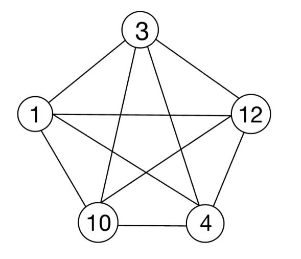
Figure 1. A simple route connection.

In Figure 1, recreational facilities are the graph’s vertices, the path is the graph’s edges, and a path’s walking time is the edge’s weight. It is a minimization problem starting and finishing at a specified vertex after having visited each other vertex exactly once, which is a traveling salesperson problem [1]

Also, there are some applications of the traveling salesperson problem. The traveling salesperson problem arises in many different contexts. This paper reports on typical applications in computer wiring, vehicle routing, clustering, and job-shop scheduling. Formulating a traveling salesperson problem is the simplest way to solve these problems. Most applications originated from real-world problems and thus seemed particularly interesting. Illustrated examples are provided with each application. [2]

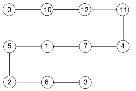
Figure 2. A Plausible Route.

Table 3. Waiting time and experiencing time.

In Figure 2, we choose the recreational facilities: TRON light cycle Power Run, Soaring over the Horizon, Rex’s Racer, Peter Pan’s flight, Seven Dwarves Mine Train, Alice in Wonderland Maze, Once Upon a Time” Adventure, Jet packs, Roaring rapids, and Slinky Dog Spin. Total time is 440minutes (waiting time) + 50minutes (experiencing time) + 121minutes (walking time) =611 minutes < 630 minutes (constraint); total satisfaction value is 71; number of recreational facility is 10 > 7 (constraint).

Limited by the constraints of total time and only one experiencing opportunity, many routes are invalid, and if we keep on listing plausible ways, it is possible to find the optimal solution.

5. Previous Formulation

5.1. Decision variables

Before we formulate the DVP problem into equations, the definition of mathematical notations and decision variables are needed:

● \( m=the number of recreational facility (7≤m≤13) \)

● \( n=the number of routes \)

● \( i=recreational facility number, i=\lbrace x|1≤x≤13,x∈z\rbrace \)

● \( j=route number, j=\lbrace x|1≤x≤n, x∈z\rbrace \)

● \( {T_{j}} \) = \( spending time of route number j \)

● \( Waiting time of recreational facility i \)

● \( {S_{i}}=the satisfaction of recreational facility i \)

● \( {T_{I}}=walking time between {i_{a }} to {i_{b}} \)

● \( {X_{j}}=1if the route is selected;0 otherwise. \)

● \( {a_{i,j}}=1if recreational facility i is part of route j; 0 otherwise. \)

5.2. Set Problem

All the attraction values are recorded in Table 2, and we must add all the attraction values of the facility that the visitor experiences. For the optimal equation, we have to maximize the total satisfaction value.

\( Maximize \) \( \lbrace 1\rbrace \) \( \sum _{i=1}^{m}{a_{ij }}{S_{i }} \) i= \( \lbrace x| 1≤x≤m,x∈z\rbrace \)

\( Subject to \) \( \lbrace 2\rbrace \) \( \sum _{i=1}^{n}{T_{j}}{X_{j}}≤6 \) 30

\( \lbrace 3\rbrace \) \( \sum _{i=1}^{m}{a_{ij}}{W_{i}}+\sum _{i=1}^{m}{a_{ij}}{T_{i}} \) +5m \( ≤630 \) , m= \( \lbrace x|7≤x≤13,x∈z\rbrace \)

In the next step, we expand the equation-add up all the attraction value

\( Maximize\lbrace 4\rbrace Z=10{a_{i}}{1_{j}} \) + \( 7{a_{i}}{2_{j}} \) +7 \( {a_{i}}{3_{j}} \) +6 \( {a_{i}}{4_{j}} \) +7 \( {a_{i}}{5_{j}} \) + \( 6{a_{i}}{6_{j}} \) +5 \( {a_{i}}{7_{j}} \) + \( 7{a_{i}}{8_{j}} \) + \( 5{a_{i}}{9_{j}} \) + \( 7{a_{i}}{10_{j}} \) + \( 9{a_{i}}{11_{j}} \) + \( 7{a_{i}}{12_{j}} \) + \( 5{a_{i}}{13_{j}} \)

\( Subject to \lbrace 5\rbrace \) \( \sum _{i=1}^{n}{T_{j}}{X_{j}}≤6 \) 30

\( \lbrace 6\rbrace \) \( \sum _{i=1}^{m}{a_{ij}}{W_{i}}+\sum _{i=1}^{m}{a_{ij}}{T_{i}} \) +5m \( ≤630 \) , m= \( \lbrace x|7≤x≤13,x∈z\rbrace \)

However, there’s something wrong with the variable, which is redundant regarding the si. It is unnecessary to count all facility’s satisfaction and sum them up just to calculate the route j’s attraction. Our professor Ming Gu made a correct and more specific equation.

5.3. Corrected Formulation

We formulate the Disney Visitor Problem (DVP) as an integer linear program (ILP). Let \( {V_{0}} \) be the entrance and \( {V_{n+1}} \) be the exit, with n being the number of attractions, and denote \( {V_{1}} \) , ··· , \( {V_{n}} \) as the attractions.

We consider the following setup:

• \( {T_{i,j}} \) is the time it takes to go from \( {V_{i}} \) to \( {V_{j}} \)

• \( {x_{i,j}} \) is the decision variable indicating whether the visitor goes from \( {V_{i}} \) to \( {V_{j}} \)

• \( {T_{j}} \) is the time it takes to play at \( {V_{j}} \)

• \( {S_{j}} \) is the satisfaction of playing at \( {V_{j}} \)

Thus,

• \( \sum _{i=0}^{n}{x_{i,j}} \) indicates whether the visitor goes to \( {V_{j}} \) , with the total satisfaction \( \sum _{j=1}^{n}{S_{j }}\sum _{i=0}^{n}{x_{i,j}} \)

• \( \sum _{j=1}^{n}{x_{0,j}} \) =1 indicates that the visitor goes to some attraction from the entrance.

• \( \sum _{i=1}^{n}{x_{i.n+1}} \) =1 indicates that the visitor leaves the exit.

• \( \sum _{i=0}^{n}{x_{i,v}} \) = \( \sum _{j=0}^{n}{x_{v,j}} \) indicates that the visitor leaves an attraction after the visit.

Putting together, we have the following ILP:

\( max \) \( \lbrace 7\rbrace \) \( \sum _{j=1}^{n}{S_{j }}\sum _{i=0}^{n}{x_{i,j}} \)

\( s.t. \lbrace 8\rbrace \sum _{j=1}^{n}{x_{0,j}}=1 \)

\( \lbrace 9\rbrace \sum _{i=1}^{n}{x_{i,n+1}}=1 \)

\( \lbrace 10\rbrace \sum _{i=0}^{n}{x_{i,v}}= \sum _{j=1}^{n+1}{x_{v,j,}} v=1,…, n \)

\( \lbrace 11\rbrace \sum _{i,j=0}^{n+1}{T_{i,j}}{x_{i,j}}+ \sum _{j=1}^{n}{T_{j}} \sum _{i=0}^{n}{x_{i,j}}≤T \)

\( {x_{i,j}}≥0, i,j=0,…., n+1 \)

We set xi,i = 0 above for all i so the visitor does not stay at any attraction after the visit.

With the first three equations, it is known that the solution will always be an integer, but for the fourth equation, we cannot make sure whether its solution is an integer. This is an integer linear program, so the solution should be integers. There may be some constraints under which our solution will always be an integer. We will use minute instead of hour as our unit to avoid situations where the solution is not an integer.

6. Improvements

● The equation that we finally corrected is precisely the [knapsack problem, which means given s set of items, each with a weight and a value, determine the number of each item included in a collection so that the total weight is less than or equal to a given limit and the total value is as significant as possible.] [3]. Here are some applications of the Knapsack problem. [In its most general form, the nonlinear knapsack problem will be defined as a nonlinear optimization problem with just one constraint, bounds on the variables, and, in some cases, a set of specially structured constraints such as generalized upper bounds (GUBs). This problem is encountered either directly or as a subproblem in a variety of applications, including production planning, financial modeling, stratified sampling, and capacity planning in manufacturing, health care, and computer networks] [4]. However, the circumstance has the limitation of time, so it is hard to solve. We must still consider whether the time congestion can be considered a time knapsack.

● The alternative method is to solve it with dynamic programming. Several items and times should be considered. It is an intractable problem, but now it is solvable.

● I want to work further on this interesting Disneyland problem(maximize enjoyment problem), [The EM (expectation-maximization) algorithm is ideally suited to problems of this sort in that it produces maximum-likelihood (ML) estimates of parameters when there is a many-to-one mapping from an underlying distribution to the distribution governing the observation. The EM algorithm is presented at a level suitable for signal-processing practitioners who have had some exposure to estimation theory.] [5] and I will talk with the Academy and learn how to take a further step with it

7. Conclusion

Our purpose is to make people maximize their satisfaction in a limited amount of time, so we focus on queuing and walking time to let them experience as many recreational facilities as possible.

References

[1]. Traveling salesperson problem https://en.wikipedia.org/wiki/Travelling_salesman_problem
[2]. Some Simple Applications of the Travelling Salesman Problem J. K. Lenstra A. H. G. Rinnooy Kan Pages 717-733 | Published online: 19 Dec 2017 https://doi.org/10.1057/jors.1975.151
[3]. Knapsack problem https://en.wikipedia.org/wiki/Knapsack_problem
[4]. The nonlinear knapsack problem – algorithms and applications Kurt M Bretthauer a, Bala Shetty Received 6 June 2000, Accepted 26 April 2001, Available online 13 January 2011. https://doi.org/10.1016/S0377-2217(01)00179-5
[5]. The expectation-maximization algorithm T.K.Moon Published in: IEEE Signal Processing Magazine (Volume: 13, Issue: 6, November 1996) Page(s): 47 - 60 Date of Publication: November 1996
Cite this article
Lin,L.;Aika,K. (2023). Disney visitor problem: Integer optimization using enumeration method and set covering problem. Theoretical and Natural Science,11,29-35.
Data availability
The datasets used and/or analyzed during the current study will be available from the authors upon reasonable request.
Disclaimer/Publisher's Note
The statements, opinions and data contained in all publications are solely those of the individual author(s) and contributor(s) and not of EWA Publishing and/or the editor(s). EWA Publishing and/or the editor(s) disclaim responsibility for any injury to people or property resulting from any ideas, methods, instructions or products referred to in the content.
About volume
Volume title: Proceedings of the 2023 International Conference on Mathematical Physics and Computational Simulation
© 2024 by the author(s). Licensee EWA Publishing, Oxford, UK. This article is an open access article distributed under the terms and
conditions of the Creative Commons Attribution (CC BY) license. Authors who
publish this series agree to the following terms:
1. Authors retain copyright and grant the series right of first publication with the work simultaneously licensed under a Creative Commons
Attribution License that allows others to share the work with an acknowledgment of the work's authorship and initial publication in this
series.
2. Authors are able to enter into separate, additional contractual arrangements for the non-exclusive distribution of the series's published
version of the work (e.g., post it to an institutional repository or publish it in a book), with an acknowledgment of its initial
publication in this series.
3. Authors are permitted and encouraged to post their work online (e.g., in institutional repositories or on their website) prior to and
during the submission process, as it can lead to productive exchanges, as well as earlier and greater citation of published work (See
Open access policy for details).