1. Introduction

Mathematical models and methods are widely used in several kinds of reality situations and are helpful in making decisions. Linear programming is one of the great mathematical methods whose requirements and constraints are represented by linear relationships. The use and purpose of using linear programming is to maximize the income or minimize the lost, which means achieve the best outcome. The application of linear programming is widely spread in numerous fields, the one that this paper will discuss is the application in solving Game theory. Game theory is the study of mathematical models of strategic interactions among rational agents, which are widely used in many fields such as social science, computer science and economics. However, for some complex situations of game theory which cannot be analyzed by mathematical methods directly, models of transformation and calculation will be needed to make them analyzable and get the satisfied payoff. The conversion depends on linear programming problem and the calculation will be solved by the algorithms related to linear programming. In that case, the development of linear programming model which can solve and analyze complex game theory and related calculation should be of important research significance. Effective linear programming model would serve as valuable reference for companies or militaries to maximize the final payoff.

The history of linear programming problem can be dated back to 1827, a method which can solve a system of solving linear inequalities was published by Fourier and was named as Fourier-Motzkin elimination [1]. After that, the development of linear programming was rapid and in 1939, a linear programming formulation and the method which can help solve general linear programming problem was carried out by soviet mathematician and economist Leonid Kantorovich [2]. The application and effect of the method lead to the plan of expenditures and returns in order to reduce expenses of the military and to increase losses imposed on the opponent [3]. The history above is a successful example of applying linear programming into non-mathematical situations to achieve the goal of best outcome in theory. Now linear programming has been widely applied in the field of optimization, most practical problems in operations research can be solved by using linear programming model [4]. Several kinds of specified cases of linear programming, such as network flow problems and multicommodity flow problems, are considered as important enough to carry out research of related algorithms and codes. Due to the significant effect of the proper utilization of linear programming, teams that can develop more advanced linear programming model will get better outcome. Therefore, the development of linear programming models which can solve complex game theory situations is of great importance.

Game theory can be divided into two general kinds: zero-sum game and non-zero-sum game. Zero-sum game involves two sides, where the income of one side must be equal to the loss of the opponent to make the sum of finial payoff be equal to zero [5]. In zero-sum situations, no cooperation and competition will appear in the relationship among the two sides which lead to the poor application, which is called a strictly competitive game [6]. In that case, non-zero-sum game can be both competitive and non- competitive which depends on the value of the sum [7]. For those kinds of complex situations, two criteria will be used to evaluate the feasibility of the model: Firstly, calculating accuracy, for example, a simple two-player zero-sum game called colonel-bolloto game, which can be commonly applied as a metaphor for electoral competition, to attract more voters to support the voters, two different political parties will put resources or money to reach the goal [8][9], a rapid enlarge will be caused as the increase of the regiments put in the battlefield and the mountains [10], Errors will be caused if the model’s calculating accuracy is not qualified. Secondly, unavoidable system Error, every model will have unavoidable calculation deviation because of the disadvantage of the system itself, system with less unavoidable deviation will be of better application.

The paper’s objective is to carry out proper models of linear programming which can be used to solve and calculate the best strategy and related best payoff in game theory. To achieve this goal, based on the limitations of zero-sum game, both zero-sum game and non-zero-sum game will be considered to make sure the model appliable in practical situations. The application of linear programming in Zero-sum game will be first be analyzed to develop the models and then non-zero-sum situations will be considered to perfect the model.

Linear systems, payoff matrix and some other mathematical tools will be used in the process. Finally, examples which are closed to reality, related data and python algorithms will be used to assess the validity and reliability of the models. The model can help provide valuable advice and insights for companies, militaries and so on, which can help make informed decisions.

2. Method

2.1. Data source

To ensure the authority and accuracy of the data source, Firstly, zero-sum-game situation will be discussed by assumption because of its low application. Secondly, for non-zero-sum game situations, both assumption and stock data collected from git-hub and TRED will be used. The websites have various data of statistics about game theory to confirm the comprehensiveness. The payoff and loss of two stock companies will be discussed and the 2020 American presidential election will be analyzed.

2.2. Zero-sum-game situations

Colonel blotto game: The background of colonel blotto is an instance of a finite two-player zero-sum game, each of Colonel Blotto and the opponent has a finite set of possible strategies, or partitions. The situation this paper will discuss have 3 mountains and 5 regiments. 6 variables will be introduced below as Table 1 and 2 show.

Table 1. Variable name and meaning.

Table 2. Variable description and range.

And because of the limit of the strategy use, one more constraint will be introduced below:

\( {x_{1}}+{x_{2}}+{x_{3}}+{x_{4}}+{x_{5}}=1 \) (1)

Next step, linear programming will be used to help solve the problem: First, the net payoff will be defined as the difference value between Colonel Blotto’s winning probability and the opponent’s. Each strategy has different ranking situations so that the probability is different, by calculating this paper can get the payoff matrix:

Table 3. Net payoff matrix.

From the data of Table 3, it can be easily explained that Colonel Blotto will focus on the minimum of each row, and the people tries to choose the row in which the minimum has the largest possible. On the other hand, the opponent will try to maximize the net payoff in each column, and the people tries to choose the column in which the maximum is the smallest possible. If Colonel Blotto plays strategy x and the opponent plays strategy y, then the net payoff to Colonel Blotto is \( {X^{T}}My \) . For every strategy x of Colonel Blotto, the opponent will select the best response:

\( β(x)= {Min_{y}} {X^{T}}y \) (2)

For every strategy y of the opponent, Colonel Blotto will select the best response:

\( α(y)= {Max_{x}}{ X^{T}}y \) (3)

When Colonel Blotto selects a strategy, the commander assumes that the opponent will select the best response. Therefore, the commander seeks \( {x^{*}} \) so that:

\( β({x^{*}})= {Max_{x}} {Min_{y }}{X^{T}}y \) (4)

The same case, the opponent will assume the same way, so that:

\( α({y^{*}})= {Min_{y}} {Max_{x}} {X^{T}}y \) (5)

2.3. Non-zero-sum game situation

Most situations are non-zero-sum games, First, this paper will do the assumption that the three instrumental variables are defined as the price. For simplicity this paper assumes that three prices can be charged by the two firms (either £3, £5 or £7), that is, three strategies are open to all competitors. Two payoff matrices are shown in Table 4 and 5.

Table 4. Payoff of Firm 1.

Table 5. Payoff of Firm 2.

This paper will use 3 variables to consider for what strategy can maximize Firm 1’s payoff (Table 6).

Table 6. The variable meaning, range and meaning.

This paper can use the same formula as zero-sum situation. In example 2, the American presidential Election will be considered, most situations voting should be considered as zero-sum, but in case of the incompletion of vote count so that the election need to be considered as non-zero-sum game.

The vote count of each state is different in the 2020 American presidential Election. To simplify the statistic in 8 states which have large population will be used to create the model.

The tables below will show the approval rating, vote counts of the two electors and the net approval rating of Joe. The objective function is to maximize Joe’s net approval rating to make sure that the elector can win the election (Table 7).

Table 7. Approval rating and net approval rating and votes.

Each elector will put resources in the states to increase their approval rating so how to arrange the resources is the problem that we need to solve, we will use variables to show that in Table 8.

In the model, we assume that the relation between the resources and the efforts is linear aggressive, which means the more resources put in the state, the higher the approval rating in the state will be it can be formulated as below.

\( {Y_{i}}=({k_{i}}+1){x_{i}}+{b_{i}} \) (6)

And the objective function is below.

\( \sum _{i=1}^{8}{∝_{i}}*{Y_{i}} \) (7)

Table 8. Variable range and description.

The constraints are shown below. Equality constraints is the sum of the resources put in should be 1, \( \sum _{i=1}^{8}{x_{i}}=1 \) . Inequality constraints is the finial approval rating should follow the range.

\( 0.374 ≤ {Y_{i}} ≤0.69 \) (8)

3. Results and discussion

3.1. Zero-sum situation

The objective function is \( {x_{0}} \) , so we can convert the game to a linear programming system: \( {x_{0}} \) need to be maximized. Subject to the constraints below, which are transferred from Table 3.

\( \begin{cases} \begin{array}{c} \frac{1}{3}{x_{2}}+\frac{1}{3}{x_{3}}+{x_{4}} +{x_{5}} ≥{x_{0}} \\ \frac{-1}{3}{x_{1}}+\frac{1}{3}{x_{4}}+\frac{2}{3}{x_{5}}≥{x_{0}} \\ \frac{-1}{3}{x_{1}}-\frac{1}{3}{x_{5}} ≥{x_{0}} \\ -{x_{1}}-\frac{1}{3}{x_{2}}+\frac{1}{3}{x_{5}} ≥{x_{0}} \\ -{x_{1}}-\frac{2}{3}{x_{2}}+\frac{1}{3}{x_{3}}-\frac{1}{3}{x_{4}}≥{x_{0}} \\ {x_{1}}+{x_{2}}+{x_{3}}+{x_{4}}+{x_{5}}=1 \end{array} \end{cases} \) (9)

For 6 variable linear programming, python algorithm will be used to help solve it: First create the objective function matrix, C = [-1, 0, 0, 0, 0, 0]. Then create the inequality constraints matrix. A = [[1, 0, -1/3, -1/3, -1, -1], [1, 1/3, 0, 0, -1/3, -2/3], [1, 1/3, 0, 0, 0, 1/3], [1, 1, 1/3, 0, 0, -1/3], [1, 1, 2/3, -1/3, 1/3, 0]] and B = [0, 0, 0, 0, 0]. Then Create the equality constraints matrix, A_eq = [0, 1, 1, 1, 1, 1], B_eq = [1], Bounds = [(None, None)*1 + (0, None)*5].

Then put the variables into the function. Res = linprog(c, A_ub = A, b_ub = B, A_eq = A_eq, b_eq = B_eq, bounds = Bounds, method = ‘simplex’). The results are shown below.

Maximum of objective function: 0. Strategy Array: [0, 0, 0, 0.5, 0.5, 0].

By analyzing it by python we can find that the finial result should be half \( {x_{3}} \) and half \( {x_{4}} \) , so the sum of \( {x_{3}} \) and \( {x_{4}} \) is 1, but if \( {x_{3}} \) = 1 or \( {x_{4}} \) = 1 the objective function value \( {x_{0}} \) is not the same. So, we can draw a diagram to find the relation between \( {x_{3}} \) , \( {x_{4}} \) and \( {x_{0}} \) : Y-axis means the value of \( {x_{0}} \) , X-axis means the value of \( {x_{3}} \) :

\( {x_{3}}+ {x_{4}}=1 \) (10)

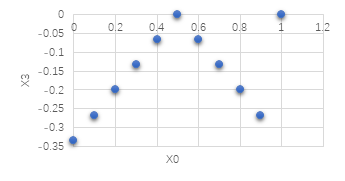
Figure 1. The relationship between X0 and X3.

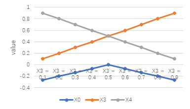
Figure 2. The trend of X0, X3 and X4.

As the Figure 1 and 4 show that when we only use strategy 3 and 4, the net payoff will increase when \( {x_{3}} \) increases from 0 to 0.5 and it will drop at the same speed when \( {x_{3}} \) increases from 0.5 to 1, which seems to be symmetric, and when \( {x_{3}} \) is equal to 1, the net payoff can also reach the maximum value.

3.2. Non-zero-sum situation

Example 1: By formulating the constraints, we can create the same pattern python code to help calculate the objective function, we will use the same function called “linprog” to make it:

Firstly, we need to calculate the objective function: S0, S1, where S0 need to be maximized. Subject to the constraints below.

\( \begin{cases} \begin{array}{c} {90S_{2}}+ 60{S_{3}}+50{S_{4}} ≥{S_{0}} \\ 150{S_{2}}+160{S_{3}}+40{S_{4}} ≥{S_{0}} \\ 180{S_{2}}+110{S_{3}}+70{S_{4}} ≥{S_{0}} \\ {S_{2}}+ {S_{3}}+ {S_{4}}=1 \end{array} \end{cases} \) (11)

S1 need to be maximized. Subject to the constraints below.

\( \begin{cases} \begin{array}{c} {-20S_{2}}-10{S_{3}}+20{S_{4}} ≥{S_{0}} \\ 30{S_{2}}+70{S_{3}}-10{S_{4}} ≥{S_{0}} \\ 120{S_{2}}+10{S_{3}}-60{S_{4}} ≥{S_{0}} \\ {S_{2}}+ {S_{3}}+ {S_{4}}=1 \end{array} \end{cases} \) (12)

By using the same python code below, the result will be easily calculated. The first step is to create the objective function matrix for calculating, C = [-1, 0, 0, 0]. Then the S0 inequality constraints matrices should be created. A = [[-1, 90, 60, 50], [-1, 150, 160, 40], [-1, 180, 110, 70]].

The S1 inequality constraints matrices should be created. A1 = [[-1, -20, -10, 20], [-1, 30, -70, -10], [-1, 120,10, -60]] and B = [0, 0, 0, 0, 0].

Finally, the equality constraints will be put into the function. A_eq = [0, 1, 1, 1], B_eq = [1], Bounds = [(None, None)*1 + (0, 1)*5], Res = linprog(c, A_ub = A, b_ub = B, A_eq = A_eq, b_eq = B_eq, bounds = Bounds, method = ‘simplex’), Res1 = linprog(c, A_ub = A1, b_ub = B, A_eq = A_eq, b_eq = B_eq, bounds = Bounds, method = ‘simplex’).

By python calculation we can get the result below. For firm 1’s payoff, the results gives that the objective function is -160.00000000000006 which means the maximum of payoff is around 160 and the X-array should be x: [1.60000000e+02, 4.99600361e-16, 1.00000000e+00, 0.00000000e+00] which gives us that we should use strategy 2 to maximize the payoff of firm 1.

For Firm 1’s net payoff it can be shown that the objective function is -120.0 and the X-array is x: [1.20000000e+02, 1.00000000e+00, 1.95399252e-14, 0.00000000e+00] which tells that strategy 1 should be used to maximize the difference value of Firm1 and Firm 2’s payoff.

3.3. Example 2

For American presidential election example. First the objective function needs to be calculated.

\( \sum _{i=1}^{8}{∝_{i}}*{Y_{i}}= 14.52{x_{1}}+69.85{x_{2}}+6.36{x_{3}}+9.9{x_{4}}+4.86{x_{5}}+5.58{x_{6}}+6.4{x_{7}}+7.11{x_{8}}+57.436 \) (13)

The constraints need to be calculated.

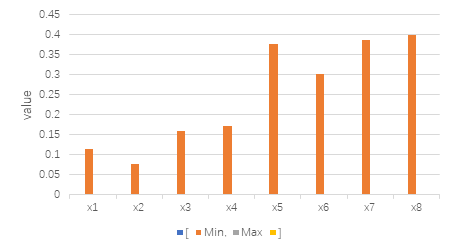
Figure 3. Variable range.

As Figure 3 shows that the range of \( {x_{5}} \) , \( {x_{7}} \) and \( {x_{8}} \) is much higher than others. After that the linprog python code will be used again to get the best optimization. The result will give us the data below. The maximum of objective function is 5.567740015157824. The x-array is [8.88701645e-11, 5.33611050e-11, 1.60000000e-01, 2.44540854e-10, 3.76000000e-01, 3.00999999e-01, 1.63000002e-01, 2.96879579e-10].

Figure 4. Each percentage of resources in the state.

From figure 4 it can be shown that only MS, KS, NV and KY need to be put in resources to maximize the approval rating while following the variable range.

4. Conclusion

The objective of this study is to investigate the application of linear programming in game theory in order to help maximize the net payoff of companies, military or politics, or minimize the loss in competition. By using the assumption such as colonel-blotto game and the data of the 2020 American presidential Election voting situations, a multiple linear programming application and relevant python codes were used to find that the resources should be put in the Washington(WA) and California(CA) most and in other states the results are close so that the influence could be ignored, in other fields like the competition and cooperation between companies could also be solved like that in the linear programming model.

References

[1]. Gerard S and Yori Z 2015 Linear and Integer Optimization: Theory and Practice (3rd ed). CRC Press.
[2]. Alexander S 1998 Theory of Linear and Integer Programming. John Wiley & Sons, 221–222.
[3]. George B D 1982 Reminiscences about the origins of linear programming. Operations Research Letters. 43–48.
[4]. Wood W K 1995 Two-person zero-sum games for network interdiction. Operations Research, 43(2), 243-251.
[5]. Chirinko B and Wilson D J 2006 State investment tax incentives: a zero-sum game? Federal Reserve Bank of San Francisco.
[6]. Francois J, Mertens S and Zamir 1971 The value of two-person zero-sum repeated games with lack of information on both sides. International Journal of Game Theory.
[7]. Zhang H, et al. 2022 Analytical and experimental nonzero-sum differential game-based control of a 7-dof robotic manipulator. Journal of Vibration and Control, 28, 707-718.
[8]. Zheng X, et al. 2022 An optimization study of provincial carbon emission allowance allocation in China based on an improved dynamic zero-sum-gains slacks-based-measure model. Sustainability.
[9]. Myerson R 1993 Incentives to cultivate favoured minorities under alternative electoral systems. American Political Science Review, 87(4), 856-869.
[10]. Laslier J F and Picard N 2002 Distributive politics and electoral competition. Journal of Economic Theory, 103, 106–130.
Cite this article
Wang,W. (2023). Linear programming and its application in analysing game theory. Theoretical and Natural Science,12,46-54.
Data availability
The datasets used and/or analyzed during the current study will be available from the authors upon reasonable request.
Disclaimer/Publisher's Note
The statements, opinions and data contained in all publications are solely those of the individual author(s) and contributor(s) and not of EWA Publishing and/or the editor(s). EWA Publishing and/or the editor(s) disclaim responsibility for any injury to people or property resulting from any ideas, methods, instructions or products referred to in the content.
About volume
Volume title: Proceedings of the 2023 International Conference on Mathematical Physics and Computational Simulation
© 2024 by the author(s). Licensee EWA Publishing, Oxford, UK. This article is an open access article distributed under the terms and
conditions of the Creative Commons Attribution (CC BY) license. Authors who
publish this series agree to the following terms:
1. Authors retain copyright and grant the series right of first publication with the work simultaneously licensed under a Creative Commons
Attribution License that allows others to share the work with an acknowledgment of the work's authorship and initial publication in this
series.
2. Authors are able to enter into separate, additional contractual arrangements for the non-exclusive distribution of the series's published
version of the work (e.g., post it to an institutional repository or publish it in a book), with an acknowledgment of its initial
publication in this series.
3. Authors are permitted and encouraged to post their work online (e.g., in institutional repositories or on their website) prior to and
during the submission process, as it can lead to productive exchanges, as well as earlier and greater citation of published work (See
Open access policy for details).