


1. Introduction
Since the 20th century, with the continuous deepening development of the concept of Industry 4.0, the complexity of manufacturing workflows has skyrocketed, and researching robots suitable for flexible production is becoming a focus of development. Industry 4.0 takes intelligent manufacturing as the leading role, improves the intelligent level of manufacturing industry, establishes a smart factory with adaptability, Resource efficiency and genetic engineering, and integrates artificial intelligence (AI), the Internet of Things (IoT), Big data, and cloud systems into existing industries and services. The era of utilizing information technology to promote industrial transformation [1-3].
In current applications, the robotic arm replaces manual labor to complete the production automation process in a fixed position [4], while the Automated Guided Vehicle (AGV) achieves automatic docking and circulation of logistics between various links. Although modern production methods have made a qualitative leap compared to traditional processing methods, the tasks that these two types of robots can accomplish still have certain limitations and cannot truly flexibly replace human labor.
Production equipment often cooperates with each other through fixed programs, only performing pre-set actions, and still experiencing the phenomenon of industrial robots discharging materials before the transfer platform reaches the designated position, which can easily cause economic losses. Fixed robotic arms can only work in limited spaces and cannot fully utilize their flexible characteristics. A single AGV can only complete a single transfer function.
With the rapid development of computer technology and sensor technology, the ability of robots to obtain their own state and environmental information has been greatly expanded. Faced with the continuous development of automation technology, the focus has shifted to independent material processing in the context of industry and manufacturing. This article proposes a robot that integrates AGV and industrial robots in future flexible manufacturing factories, possessing environmental perception ability, optimal decision-making ability, and autonomous operation ability, as well as functions such as mobile transportation, flexible operation, human-machine interaction and cooperation. Integrated systems can improve material supply efficiency and robustness between machines.
2. Methodology
2.1. Modern industrial production methods
With the advancement of automation level, more and more industries are transitioning from labor-intensive to intelligent and flexible production, and AGVs and industrial robots are also increasingly being applied in practical production on a large scale. The emergence of AGVs has gradually replaced manual forklift handling between production lines, while the emergence of industrial robots has changed the current situation where traditional production lines can only produce a single item.
2.1.1. Introduction of AGVs. Intelligent transportation is an important component of the development plan for the new generation of artificial intelligence, and AGV, as a type of intelligent transportation, also plays a crucial role. In order to reduce labor costs, unmanned warehousing and intelligent AGVs have gradually become research hotspots. Most modern AGVs use electromagnetic induction technology, laser detection technology, optical detection technology, Ultrasonic testing technology, etc. for positioning and navigation. Need to train scheduling models based on the new work environment [5].
With the development of artificial intelligence and AGV technology, AGV has been applied to more and more scenarios, mainly including factories, logistics, supermarkets, hospitals, and parking lots. AGV can cooperate with assembly workers on the production line in the factory for partial transfer work, taking into account the convenience of fast transportation and worker operation. Each AGV in the control system is both interrelated and relatively independent. If a certain AGV in the system fails, the backup AGV can be quickly withdrawn or replaced, thereby restoring system operation and greatly reducing fault repair time. By flexibly increasing or decreasing the number of AGVs in the system, or adjusting the operating speed of AGVs, the goal of adapting to different production rhythms can be achieved. Therefore, AGV systems have strong flexibility. In addition, compared to manual delivery, it improves the accuracy and timeliness of material delivery, avoids path conflicts caused by communication issues during manual forklift transportation, improves delivery efficiency, and reduces labor costs.
2.1.2. Introduction of industrial robots. Industrial robots have replaced traditional manual heavy work activities. In actual production, industrial robots can carry out processing tasks according to established computer control programs. Compared to traditional manual production lines, it eliminates the processing problems that may arise from fatigue and distraction during manual production. Not only did it liberate labor, but it also improved processing accuracy and production quality. Another major advantage of industrial robot production is strong production flexibility and wider adaptability. Traditional production lines are expensive and mostly customized to produce a specific product, making it impossible for multiple products to share a single production line [6]. The emergence of industrial robots allows the same production line to quickly switch between the products that need to be produced during production.
2.2. Design of AGV combining with industrial robots
This article proposes a transfer AGV with an industrial robotic arm, attempting to propose a new application solution for the final step of the production line's cutting and transfer work. The industrial robots on AGV can replace manual labor or specially designed loading and unloading devices, further improving the flexibility of the production line. The chassis of this AGV is equipped with Simultaneous Localization and Mapping (SLAM) device, which can autonomously plan and navigate the path, and can automatically avoid moving workers or accidentally falling goods in the factory. Further reducing manual intervention in flexible production.
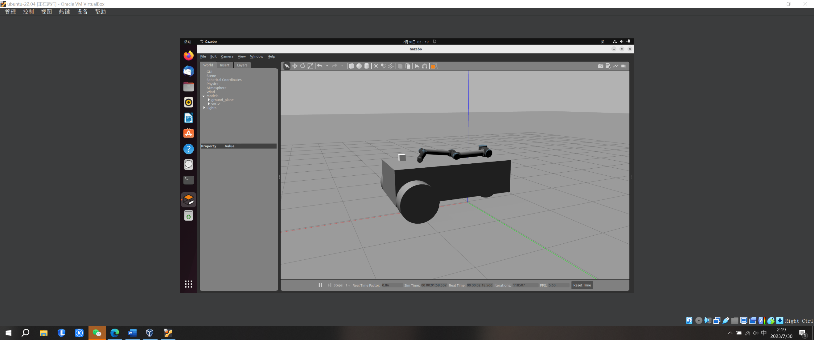
The initial design idea of this article was to create a mobile industrial robotic arm on the AGV platform based on the Robot Operating System (ROS) system. This article retrieved relevant information and designed the following car model with a robotic arm using Gazebo for simulation experimental research.
The robot includes a LiDAR, an AGV chassis with cargo carrying capacity, and a multi degree of freedom robotic arm. In terms of sensors, Velodye in Gazebo was selected_ Simulator LiDAR. In terms of the robotic arm, Universal Robotics' open-source UR10 robotic arm was used, greatly reducing the time for model production. The six degrees of freedom of the robotic arm well met the preliminary design requirements. The robot structure in the Gazebo environment is shown in Figure 1 below.
|
Figure 1. Designed robot structure. |
2.2.1. Mechanical arm design. This article adopts the UR10 industrial robot as the design of the robotic arm to complete grasping or operating tasks. UR10 industrial manipulator is a series industrial robot with Six degrees of freedom. The rated load is 10Kg, and the radius of the specified working range can reach 1300mm. All six joints of the manipulator are rotary joints. The end actuator of the manipulator can change different processing tools for different working conditions, which is suitable for a variety of processing and manufacturing environments.
The D-H parameter method is the most commonly used Kinematics analysis method for robots at present. The advantage of this method is that regardless of the degree of freedom and complexity of the structure of the robotic arm, as long as it can be simplified as a linkage mechanism, it can express the position and pose of the manipulator, so as to establish a mathematical model of Kinematics. According to the above standard D-H parameter method. As shown in Figure 2, the corresponding linkage coordinate system is established for the UR10 industrial robotic arm [7].
|
Figure 2. Coordinate system of UR10 robotic arm [8]. |
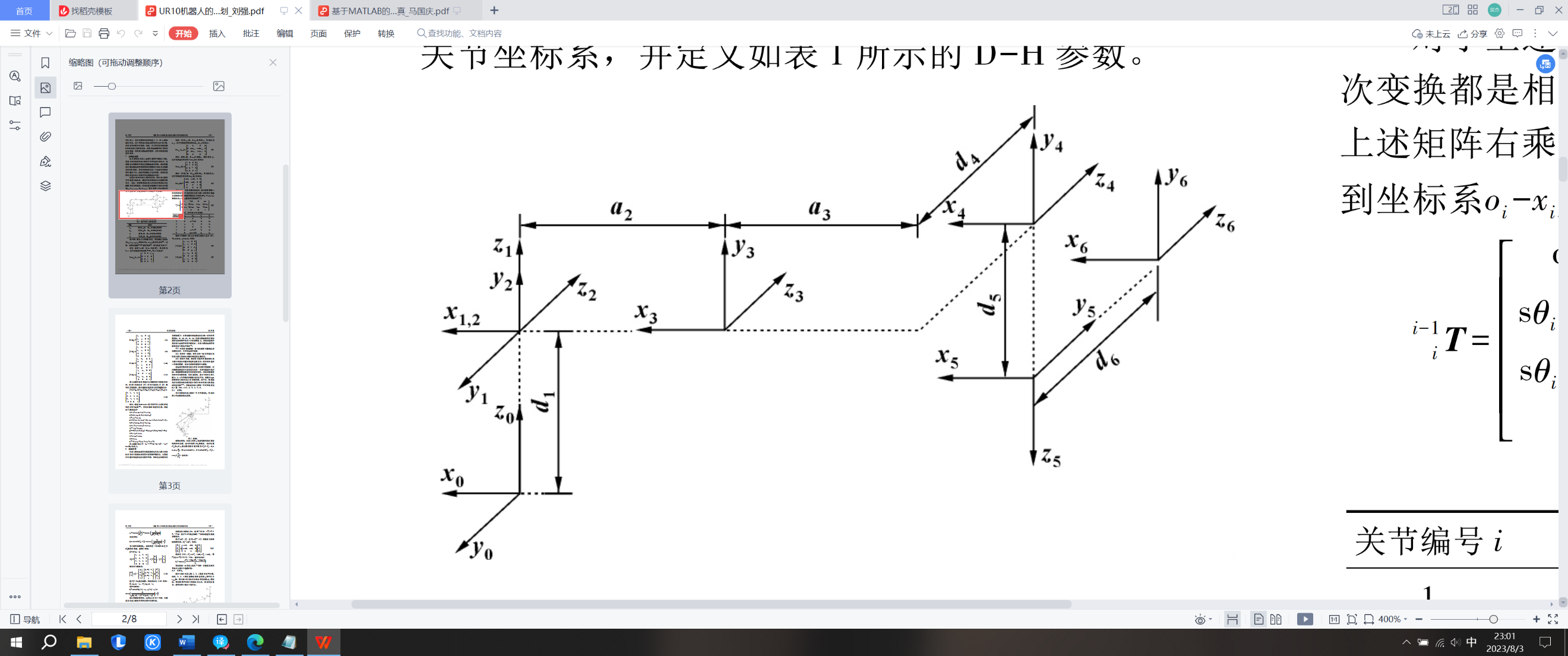
The DH method requires defining a coordinate system for each joint to determine the coordinate transformation between adjacent coordinate systems. The D-H parameter definition of the UR10 robotic arm is shown in Table 1.
Table 1. Link D-H parameter definition. | |
parameter | illustrate |
\( {a_{i-1}} \) | Moving distance from \( {z_{i-1}} \) to \( {z_{i}} \) along the \( {x_{i-1}} \) axis |
\( {α_{i-1}} \) | Torsional angle from \( {z_{i-1}} \) to \( {z_{i}} \) around the \( {x_{i-1}} \) axis |
\( {d_{i}} \) | The displacement from \( {x_{i-1}} \) to \( {x_{i}} \) along the \( {z_{i}} \) axis |
\( {θ_{i}} \) | Rotate from \( {x_{i-1}} \) to the corner of \( {x_{i}} \) around the \( {z_{i}} \) axis |
According to Figure 2 and Table 1, the D-H parameters of the UR10 robotic arm link can be obtained, as shown in Table 2.
Table 2. UR10 industrial robot D-H parameters. | |||||
Joint | Link Twist | Link Length | Link Offset | Joint Angle | Joint Range |
\( {(α_{i-1}}/°) \) | \( {(a_{i-1}}/mm) \) | \( ({d_{i}}/mm) \) | \( ({θ_{i}}/°) \) | ||
\( {J_{1}} \) | 0 | 0 | \( {d_{1}} \) | \( {θ_{1}} \) | \( ±360° \) |
\( {J_{2}} \) | 90 | 0 | 0 | \( {θ_{2}} \) | \( ±360° \) |
\( {J_{3}} \) | 0 | \( {a_{2}} \) | 0 | \( {θ_{3}} \) | \( ±360° \) |
\( {J_{4}} \) | 0 | \( {a_{3}} \) | \( {d_{4}} \) | \( {θ_{4}} \) | \( ±360° \) |
\( {J_{5}} \) | 90 | 0 | \( {d_{5}} \) | \( {θ_{5}} \) | \( ±360° \) |
\( {J_{6}} \) | -90 | 0 | \( {d_{6}} \) | \( {θ_{6}} \) | \( ±360° \) |
The following equation is a Kinematics analysis of the manipulator. In Robotics, the movement of a manipulator can be regarded as the translation and rotation of a rigid link. For transformation from coordinate system \( \lbrace n\rbrace \) to coordinate system \( \lbrace n+1\rbrace \) . The following conditions are required. First, space coordinate system translation transformation matrix: \( Trans(0,0,{d_{n+1}}) \) and \( Trans({a_{n+1}},0,0) \) ; Second, the rotation transformation matrix can be represented as \( Rot(z,{θ_{n+1}}) \) , \( Rot(x,{α_{n+1}}) \) . Finally, the total transformation matrix \( {A_{n+1}} \) is represented as:
\( {A_{n+1}}=Rot(z,{θ_{n+1}})×Trans(0,0,{d_{n+1}})×Trans({a_{n+1}},0,0)×Rot(x,{α_{n+1}}) \) \( =[\begin{matrix}c{θ_{n+1}} & -s{θ_{n+1}} & 0 & 0 \\ s{θ_{n+1}} & c{θ_{n+1}} & 0 & 0 \\ 0 & 0 & 1 & 0 \\ 0 & 0 & 0 & 1 \\ \end{matrix}][\begin{matrix}1 & 0 & 0 & 0 \\ 0 & 1 & 0 & 0 \\ 0 & 0 & 1 & {d_{n+1}} \\ 0 & 0 & 0 & 1 \\ \end{matrix}][\begin{matrix}1 & 0 & 0 & {a_{n+1}} \\ 0 & 1 & 0 & 0 \\ 0 & 0 & 1 & 0 \\ 0 & 0 & 0 & 1 \\ \end{matrix}][\begin{matrix}1 & 0 & 0 & 0 \\ 0 & c{α_{n+1}} & -s{α_{n+1}} & 0 \\ 0 & s{α_{n+1}} & c{α_{n+1}} & 0 \\ 0 & 0 & 0 & 1 \\ \end{matrix}] \) \( =[\begin{matrix}c{θ_{n+1}} & -s{θ_{n+1}}c{α_{n+1}} & s{θ_{n+1}}s{α_{n+1}} & {a_{n+1}}c{θ_{n+1}} \\ s{θ_{n+1}} & c{θ_{n+1}}c{α_{n+1}} & -c{θ_{n+1}}s{α_{n+1}} & {a_{n+1}}s{θ_{n+1}} \\ 0 & s{α_{n+1}} & c{α_{n+1}} & {d_{n+1}} \\ 0 & 0 & 0 & 1 \\ \end{matrix}] \) | (1) |
The forward Kinematics model of the manipulator has been established according to the DH parameter table, and the transformation matrix between any two connecting rods is:
\( {^R}{T_{H}}={^R}T_{1}^{1}T_{2}^{2}{T_{3}}⋯{^n-1}{T_{n}} \) | (2) |
By combining formulas (1) and (2), the ratio of adjacent two connecting rods can be obtained. The general formula for inter pose transformation is:
\( {^i-1}{T_{i}}=[\begin{matrix}c{θ_{i}} & -s{θ_{i}}c{α_{i-1}} & s{θ_{i}}s{α_{i-1}} & {a_{i-1}}c{θ_{i}} \\ s{θ_{i}} & c{θ_{i}}c{α_{i-1}} & -c{θ_{i}}s{α_{i-1}} & {a_{i-1}}s{θ_{i}} \\ 0 & s{α_{i-1}} & c{α_{i-1}} & {d_{i}} \\ 0 & 0 & 0 & 1 \\ \end{matrix}] \) | (3) |
Thus, the forward Kinematics equation of UR industrial robot is established.
In order to plan the trajectory of the manipulator, Inverse kinematics should also be introduced. The Inverse kinematics theory of the industrial manipulator is solved, that is, the position and orientation of its end relative to the base coordinate are known, and the values of each joint variable of the industrial manipulator are solved. In the daily use of industrial manipulator, its motion track is determined and known. At this time, in order to control the manipulator to achieve the expected motion, it is necessary to solve the corresponding joint variables by using the Inverse kinematics of the manipulator. For UR10 industrial manipulator, in order to control it to complete the task, it is necessary to use Inverse kinematics to solve the corresponding six joint angles, and then input the joint motion variables into the controller, so that the manipulator can further complete the task according to the expected trajectory.
The forward Kinematics solution of the UR10 industrial manipulator is unique, and its Inverse kinematics solution is not unique. To complete the inverse kinematics analysis of the industrial manipulator is a necessary prerequisite for the manipulator to carry out motion trajectory planning, so solving the Inverse kinematics problem is of great significance. Because the second, third, and fourth rotation joint axes of the UR10 industrial robot all meet the parallel spatial relationship, and meet the spatial position conditions of three adjacent rotation joint axes being parallel or intersecting, the inverse Kinematics solution of the UR10 industrial manipulator exists. In this chapter, Paul algebraic method is used to solve the Inverse kinematics of the manipulator.
\( {θ_{1}}=arctan{(\frac{{P_{y}}}{{P_{x}}})}-arctan\frac{{({d_{2}}+{d_{3}})^{2}}}{±\sqrt[]{{r^{2}}-{({d_{2}}+{d_{3}})^{2}}}} \) | (4) |
\( {θ_{2}}=arctan\frac{{c_{1}}{o_{x}}+{s_{1}}{o_{y}}+{c_{5}}{c_{6}}\frac{{c_{2}}{a_{x}}+{s_{1}}{a_{y}}}{{s_{5}}}+{c_{6}}\frac{{a_{z}}}{{s_{5}}}}{{o_{z}}-{c_{6}}\frac{{c_{1}}{a_{x}}+{s_{1}}{a_{y}}}{{s_{5}}}{c_{5}}{c_{6}}\frac{{a_{z}}}{{s_{5}}}} \) | (5) |
\( {θ_{3}}=arctan(\frac{-{c_{1}}{s_{2}}{p_{x}}-{s_{1}}{s_{2}}{p_{y}}-{c_{2}}{p_{z}}+{d_{5}}\frac{{c_{1}}{c_{2}}{a_{z}}+{s_{1}}{c_{2}}{a_{y}}-{s_{2}}{a_{z}}}{{s_{5}}}}{{a_{3}}}) \) | (6) |
\( {θ_{4}}=arcsin{(\frac{-{a_{z}}}{{s_{5}}})}-arctan\frac{{c_{1}}{o_{x}}+{s_{1}}{o_{y}}+{c_{5}}{c_{6}}\frac{{c_{1}}{a_{x}}+{s_{1}}{a_{y}}}{{s_{5}}}+{c_{6}}\frac{{a_{z}}}{{s_{5}}}}{{o_{z}}-{c_{6}}\frac{{c_{1}}{a_{x}}+{s_{1}}{a_{y}}}{{s_{5}}}+{c_{5}}{c_{6}}\frac{{a_{z}}}{{s_{5}}}} \) | (7) |
\( {θ_{5}}=arccos({s_{1}}{a_{x}}-{c_{1}}{a_{y}}) \) | (8) |
\( {θ_{6}}=arccos(\frac{{c_{1}}{n_{y}}-{s_{1}}{n_{x}}}{{s_{5}}}) \) | (9) |
\( r=\sqrt[]{{{p_{x}}^{2}}+{{p_{y}}^{2}}} \) | (10) |
2.2.2. Mobile chassis design. In the chassis motion mode, this article selects a two wheel differential chassis. The two wheel differential chassis is a widely used robot chassis that provides power through two driving wheels and turns based on the speed difference between the tires on both sides. The universal wheels on the back of the chassis can keep the robot balanced. The differential chassis can rotate in place, which is highly flexible and has simple and effective control methods. Moreover, its cost is low, making it widely used [9].
Next, the AGV chassis is analyzed in Kinematics. Two basic wheel Kinematics constraints are proposed for the chassis tire: rolling constraint, when the motion occurs in the proper direction, the wheel must roll; Sliding constraint, there should be no lateral sliding, and the wheels should not slide perpendicular to the plane of the wheels.
Rigid-body rotating at angular velocity \( ω \) analysis:
𝑉𝐴=𝑉𝑃+𝜔×𝑟𝐴/𝑃 | (11) |
This produces two constraints on the robot linear ( \( {V_{P}} \) ) and angular ( \( ω \) ) velocities:
𝑟𝑜𝑙𝑙𝑖𝑛𝑔:𝑡∙𝑉𝑃+𝑡∙𝜔×𝑟𝐴𝑃=𝑡∙𝑉𝐴=𝑟𝜑 | (12) |
\( sliding:\hat{n}∙{V_{P}}+\hat{n}∙ω×{r_{\frac{A}{P}}}=\hat{n}∙{V_{A}}=0 \) | (13) |
The sliding constraint reduces the mobility by one. Evaluate the above expression in terms of \( α,β,ω=ωk, and {V_{P}}=ui+vj \)
\( rolling:usin(α+β)-vcos{(α+β)}-ωlcosβ=r\dot{φ} \) | (14) |
\( sliding:ucos(α+β)-vsin{(α+β)}+ωlsinβ=0 \) | (15) |
Thus, forward Kinematics can be abstracted:
\( [\begin{matrix}\dot{{φ_{L}}} \\ \dot{{φ_{R}}} \\ \end{matrix}]=\frac{1}{r}[\begin{matrix}1 & -l \\ 1 & l \\ \end{matrix}][\begin{matrix}v \\ ω \\ \end{matrix}] \) | (16) |
Coordinate transformation:
\( \dot{x}=vcosθ, \dot{y}=vsinθ \) | (17) |
The differential Kinematics equation is as follows:
\( [\begin{matrix}\dot{x} \\ \dot{y} \\ \dot{z} \\ \end{matrix}]=[\begin{matrix}cos{θ} & 0 \\ sin{θ} & 0 \\ 0 & 1 \\ \end{matrix}][\begin{matrix}ν \\ ω \\ \end{matrix}]=[\begin{matrix}cos{θ} & 0 \\ sin{θ} & 0 \\ 0 & 1 \\ \end{matrix}][\begin{matrix}\frac{r}{2}(\dot{{φ_{r}}}+\dot{{φ_{l}}}) \\ \frac{r}{2d}(\dot{{φ_{r}}}-\dot{{φ_{l}}}) \\ \end{matrix}] \) | (18) |
3. Simulation results and analysis
3.1. Simulation setting
The predecessor of ROS2 was ROS, which is the Robot Operating System. The emergence of Ros solved the communication problem of various components of robots, and later more and more robot algorithms were integrated into ROS. ROS simplifies the difficulty of creating complex robots on various robot platforms and simplifies the initial effort invested by research teams in platform construction, that is, when implementing a certain function, it can be directly used or modified. Before ROS, coordinating and communicating various parts of a robot was a very complex task. ROS2 inherited ROS, which is more powerful and excellent compared to ROS. The system architecture has undergone disruptive changes: all nodes in ROS1 need to work under the management of the node manager ROS Master. Once the Master encounters problems, the system faces the risk of downtime. ROS2 has achieved true distribution and no longer has the role of Master. With the help of a new communication framework DDS, it provides reliable guarantee for communication among all nodes. Therefore, ROS2 was selected for application in the simulation validation of this article [10].
Gazebo is a three-dimensional robot simulation software that can accurately and efficiently simulate high-fidelity physical models. As a Open-source software, it can accurately and efficiently simulate the ability of robots to work in complex environments, providing a high-level simulation platform for developers. In addition, this software has good compatibility with ROS, not only simulating the appearance of robots, but also detecting collisions of objects.
Matrix Laboratory (MATLAB) is an advanced interactive numerical calculation and visualization software widely used in fields such as data analysis, image processing, algorithm development, deep learning, and robotics. It has strong scalability and provides an efficient computing platform for scientific research, engineering design, and many complex problems that require numerical calculations [11].
3.2. Simulation results
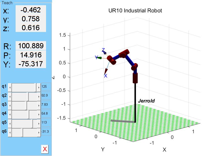
3.2.1. Manipulator grasping operation. In order to verify whether the mathematical relationship derived above is correct, Kinematics simulation of the robot is carried out using Robotics Toolbox [12], based on the data provided in Table 1. The simulation of the UR10 robot is shown in Figure 3.
|
Figure 3. Robot arm control interface. |
The position, velocity, acceleration variation curve, and trajectory planning function in joint space obtained after setting the translation action of the robotic arm are shown in Figure 4.
|
|
(a) | (b) |
|
|
(c) | (d) |
Figure 4. Trajectory planning in joint space of robotic arms. (a) is position change curve; (b) is speed variation curve; (c) is acceleration variation curve; (d) is trajectory curve in joint space. | |
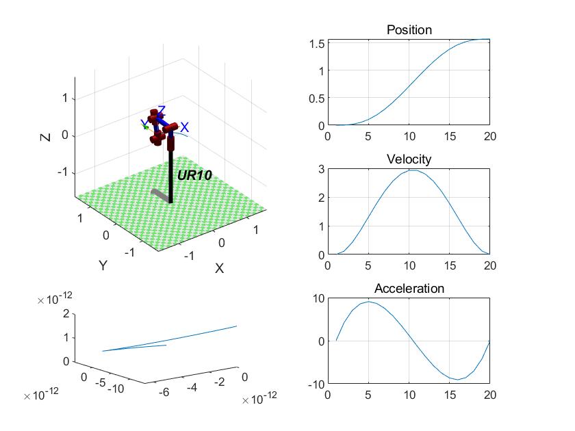


Figure 4 shows that the robotic arm can achieve smooth trajectory motion in joint space simulated by MATLAB.
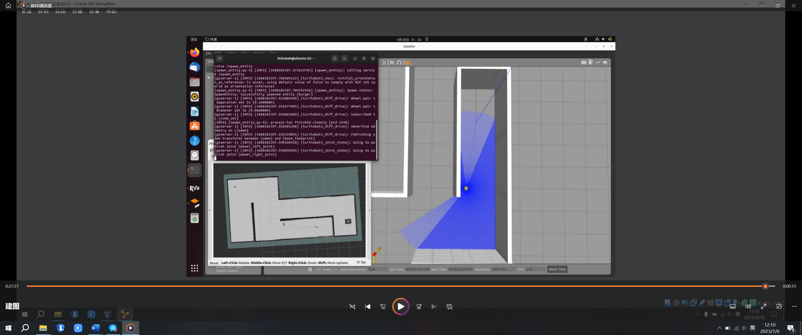
3.2.2. Mobile trajectory planning in simulation environment. This article establishes multiple factory environment models in Gazebo to test whether robots have the ability to perceive the environment, make optimal decisions, and operate independently during the production process. The established factory environment model is shown in Figure 5.
|
Figure 5. Gazebo simulated factory environment. |
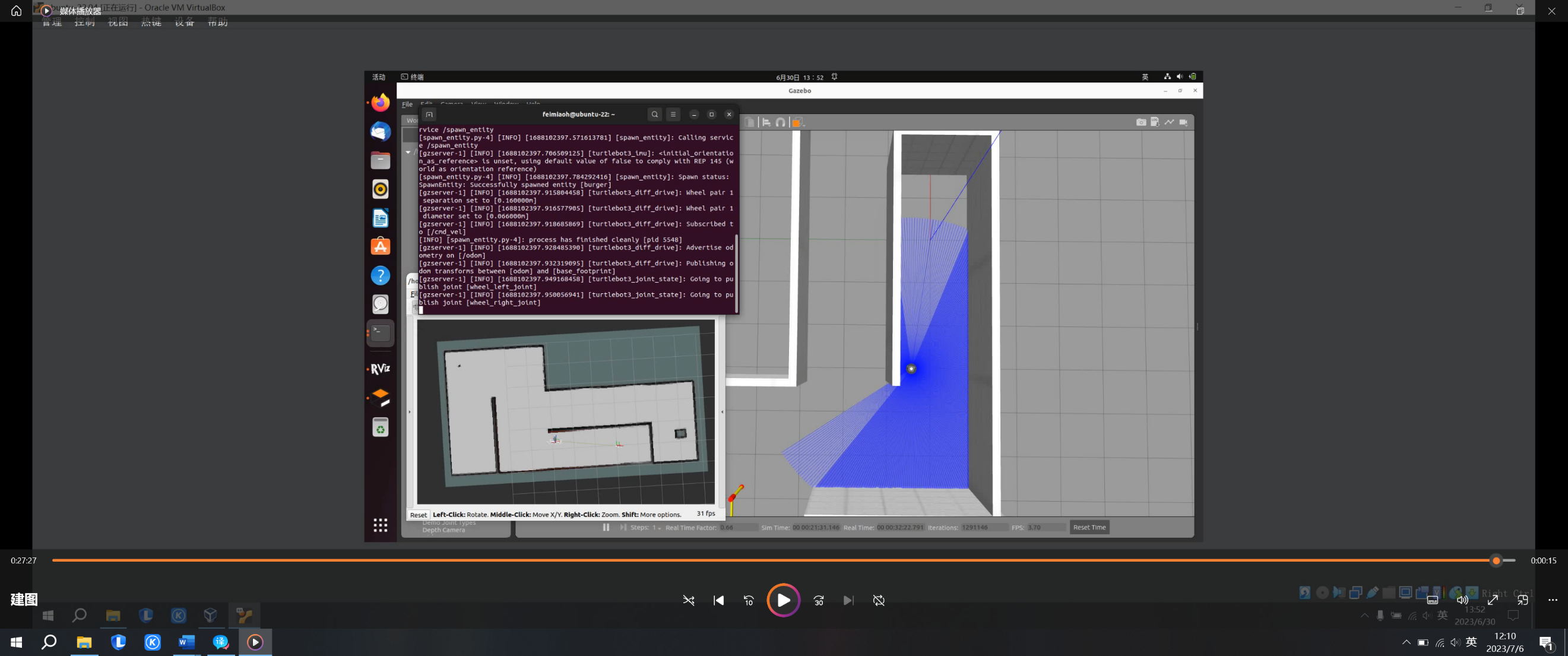
Because this article uses a differential chassis design similar to Turtlebot3, they have the same Kinematics function. Therefore, in order to test the robot's road force planning ability more efficiently, the map building and path planning functions in the new factory environment are tested on the basis of Turtlebot3 model. TurtleBot3 is a cost-effective mobile robot based on ROS, widely used in education, research, and product prototype manufacturing, which can be used for education, research, and product prototype manufacturing [13].
The first step in making robots move automatically is to draw an environmental map. SLAM is the main technology for building maps, which has multiple components: landmark extraction; Data association; State estimation; Status updates and coordinate updates. Build SLAM maps by using Cartographer. After starting the simulation environment, start the mapper, and then control the robot to draw a map through the keyboard. After the map construction is completed, save the map results as shown in Figure 6:
|
Figure 6. SLAM map results. |
The navigation framework uses Navigation2. Navigation2 has three mobile servers: recovery server, controller server and planner server. The Planning Server can calculate the shortest path along a predefined route and use the A* algorithm for path planning. Recovery Server can handle unknown or faulty situations in the system's processing system. When a robot is stuck due to dynamic obstacles or poor control status, it can be allowed to move from a harsh position to a free space where it can successfully navigate by reversing or rotating in place.
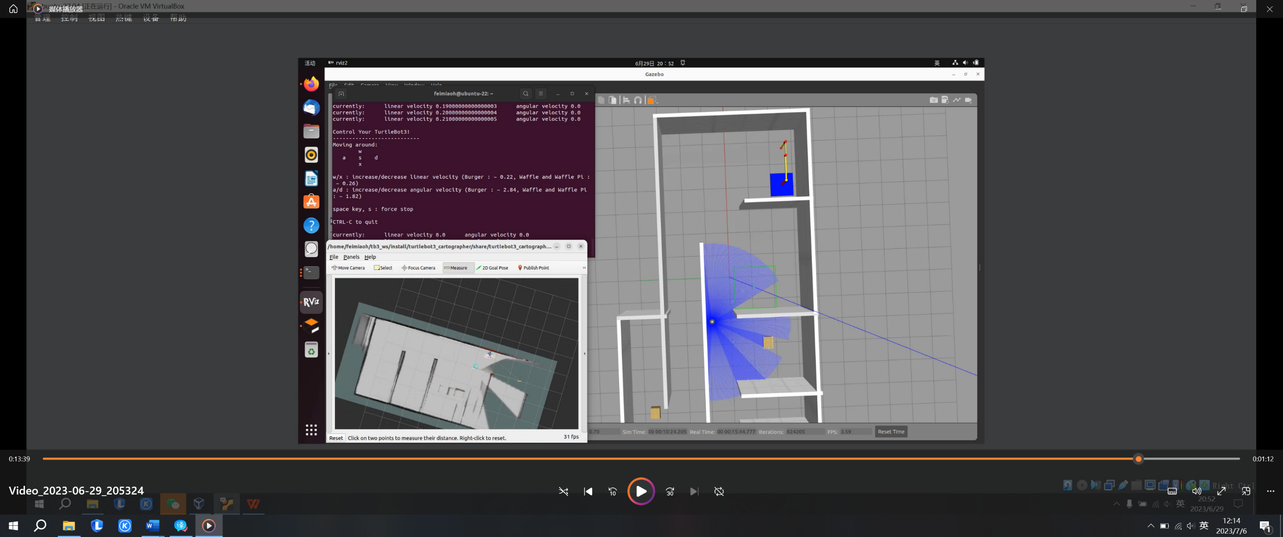
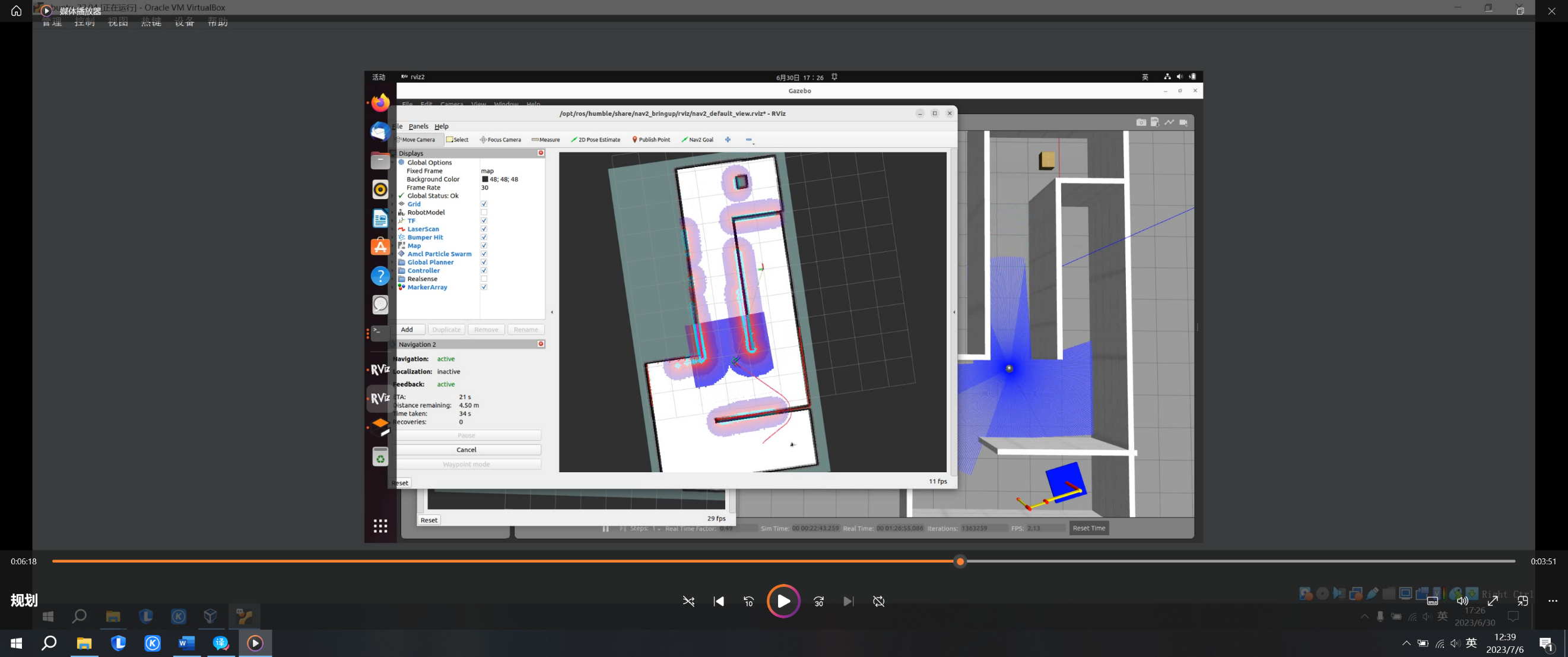
In a planning simulation experiment, the robot mistakenly regarded walls that were not explored during the pre-SLAM map establishment process as passable paths, but found that this was an insurmountable obstacle during autonomous navigation, as shown in Figure 7. a. However, soon the robot autonomously replanned a feasible path, as shown in Figure 7. b.
|
|
(a) | (b) |
Figure 7. Path planning demonstration. | |

4. Conclusion
In order to comply with the intelligent production requirements of Industry 4.0, this article designs a flexible production robot that combines AGV with industrial robots. It has the ability to perceive the environment, make the best decisions, and operate independently. This article uses Gazebo to construct a production environment and simulates the motion of robots. In addition, simulation experiments were conducted on the operation of the UR10 robot using MATLAB. It has been verified that the robot can achieve functions such as mobile transportation, flexible operation, human-machine interaction and collaboration on the production line.
After testing in the Gazebo factory environment, the result of the robot moving from the production line to the part storage location was: the shortest path length was 12.08 meters, and the path required time was 59 seconds. The experimental results and planning path map validate the feasibility and effectiveness of this method. The mobile robot designed in this article combines a robotic arm with an AGV, hoping to have certain application value in future flexible manufacturing factories.
References
[1]. Hana Neradilova, Gabriel Fedorko, Simulation of the Supply of Workplaces by the AGV in the Digital Factory, Procedia Engineering, Volume 192, 2017, Pages 638-643, ISSN 1877-7058
[2]. Cupek, R. et al. (2020). Autonomous Guided Vehicles for Smart Industries – The State-of-the-Art and Research Challenges. In: Krzhizhanovskaya, V.V., et al. Computational Science – ICCS 2020. ICCS 2020. Lecture Notes in Computer Science(), vol 12141. Springer, Cham. https://doi.org/10.1007/978-3-030-50426-7_25
[3]. Lucas Santos Dalenogare, Guilherme Brittes Benitez, Néstor Fabián Ayala, Alejandro Germán Frank, The expected contribution of Industry 4.0 technologies for industrial performance, International Journal of Production Economics, Volume 204, 2018, Pages 383-394, ISSN 0925-5273, https://doi.org/10.1016/j.ijpe.2018.08.019.
[4]. Zengxi Pan, Joseph Polden, Nathan Larkin, Stephen Van Duin, John Norrish, Recent progress on programming methods for industrial robots, Robotics and Computer-Integrated Manufacturing, Volume 28, Issue 2, 2012, Pages 87-94, ISSN 0736-5845
[5]. C. Wang and J. Mao, "Summary of AGV Path Planning," 2019 3rd International Conference on Electronic Information Technology and Computer Engineering (EITCE), Xiamen, China, 2019, pp. 332-335, doi: 10.1109/EITCE47263.2019.9094825.
[6]. Arents, J.; Greitans, M. Smart Industrial Robot Control Trends, Challenges and Opportunities within Manufacturing. Appl. Sci. 2022, 12, 937. https://doi.org/10.3390/app12020937
[7]. C.R. Rocha, C.P. Tonetto, A. Dias, A comparison between the Denavit–Hartenberg and the screw-based methods used in kinematic modeling of robot manipulators, Robotics and Computer-Integrated Manufacturing, Volume 27, Issue 4, 2011, Pages 723-728, ISSN 0736-5845, https://doi.org/10.1016/j.rcim.2010.12.009.
[8]. Q. Liu, D. Yang, W. Hao and Y. Wei, "Research on Kinematic Modeling and Analysis Methods of UR Robot," 2018 IEEE 4th Information Technology and Mechatronics Engineering Conference (ITOEC), Chongqing, China, 2018, pp. 159-164, doi: 10.1109/ITOEC.2018.8740681.
[9]. Shojaei, K., Shahri, A., Tarakameh, A., & Tabibian, B. (2011). Adaptive trajectory tracking control of a differential drive wheeled mobile robot. Robotica, 29(3), 391-402. doi:10.1017/S0263574710000202
[10]. Steven Macenski et al. ,Robot Operating System 2: Design, architecture, and uses in the wild.Sci. Robot.7,eabm6074(2022).DOI:10.1126/scirobotics.abm6074
[11]. Eric A. Sobie ,An Introduction to MATLAB.Sci. Signal.4,tr7-tr7(2011).DOI:10.1126/scisignal.2001984
[12]. P. I. Corke, "A robotics toolbox for MATLAB," in IEEE Robotics & Automation Magazine, vol. 3, no. 1, pp. 24-32, March 1996, doi: 10.1109/100.486658.
[13]. Amsters, R., Slaets, P. (2020). Turtlebot 3 as a Robotics Education Platform. In: Merdan, M., Lepuschitz, W., Koppensteiner, G., Balogh, R., Obdržálek, D. (eds) Robotics in Education. RiE 2019. Advances in Intelligent Systems and Computing, vol 1023. Springer, Cham. https://doi.org/10.1007/978-3-030-26945-6_16
Cite this article
Tai,J. (2024). A design of intelligent AGV system combined with a robotic arm for flexible production lines. Applied and Computational Engineering,34,84-94.
Data availability
The datasets used and/or analyzed during the current study will be available from the authors upon reasonable request.
Disclaimer/Publisher's Note
The statements, opinions and data contained in all publications are solely those of the individual author(s) and contributor(s) and not of EWA Publishing and/or the editor(s). EWA Publishing and/or the editor(s) disclaim responsibility for any injury to people or property resulting from any ideas, methods, instructions or products referred to in the content.
About volume
Volume title: Proceedings of the 2023 International Conference on Machine Learning and Automation
© 2024 by the author(s). Licensee EWA Publishing, Oxford, UK. This article is an open access article distributed under the terms and
conditions of the Creative Commons Attribution (CC BY) license. Authors who
publish this series agree to the following terms:
1. Authors retain copyright and grant the series right of first publication with the work simultaneously licensed under a Creative Commons
Attribution License that allows others to share the work with an acknowledgment of the work's authorship and initial publication in this
series.
2. Authors are able to enter into separate, additional contractual arrangements for the non-exclusive distribution of the series's published
version of the work (e.g., post it to an institutional repository or publish it in a book), with an acknowledgment of its initial
publication in this series.
3. Authors are permitted and encouraged to post their work online (e.g., in institutional repositories or on their website) prior to and
during the submission process, as it can lead to productive exchanges, as well as earlier and greater citation of published work (See
Open access policy for details).
References
[1]. Hana Neradilova, Gabriel Fedorko, Simulation of the Supply of Workplaces by the AGV in the Digital Factory, Procedia Engineering, Volume 192, 2017, Pages 638-643, ISSN 1877-7058
[2]. Cupek, R. et al. (2020). Autonomous Guided Vehicles for Smart Industries – The State-of-the-Art and Research Challenges. In: Krzhizhanovskaya, V.V., et al. Computational Science – ICCS 2020. ICCS 2020. Lecture Notes in Computer Science(), vol 12141. Springer, Cham. https://doi.org/10.1007/978-3-030-50426-7_25
[3]. Lucas Santos Dalenogare, Guilherme Brittes Benitez, Néstor Fabián Ayala, Alejandro Germán Frank, The expected contribution of Industry 4.0 technologies for industrial performance, International Journal of Production Economics, Volume 204, 2018, Pages 383-394, ISSN 0925-5273, https://doi.org/10.1016/j.ijpe.2018.08.019.
[4]. Zengxi Pan, Joseph Polden, Nathan Larkin, Stephen Van Duin, John Norrish, Recent progress on programming methods for industrial robots, Robotics and Computer-Integrated Manufacturing, Volume 28, Issue 2, 2012, Pages 87-94, ISSN 0736-5845
[5]. C. Wang and J. Mao, "Summary of AGV Path Planning," 2019 3rd International Conference on Electronic Information Technology and Computer Engineering (EITCE), Xiamen, China, 2019, pp. 332-335, doi: 10.1109/EITCE47263.2019.9094825.
[6]. Arents, J.; Greitans, M. Smart Industrial Robot Control Trends, Challenges and Opportunities within Manufacturing. Appl. Sci. 2022, 12, 937. https://doi.org/10.3390/app12020937
[7]. C.R. Rocha, C.P. Tonetto, A. Dias, A comparison between the Denavit–Hartenberg and the screw-based methods used in kinematic modeling of robot manipulators, Robotics and Computer-Integrated Manufacturing, Volume 27, Issue 4, 2011, Pages 723-728, ISSN 0736-5845, https://doi.org/10.1016/j.rcim.2010.12.009.
[8]. Q. Liu, D. Yang, W. Hao and Y. Wei, "Research on Kinematic Modeling and Analysis Methods of UR Robot," 2018 IEEE 4th Information Technology and Mechatronics Engineering Conference (ITOEC), Chongqing, China, 2018, pp. 159-164, doi: 10.1109/ITOEC.2018.8740681.
[9]. Shojaei, K., Shahri, A., Tarakameh, A., & Tabibian, B. (2011). Adaptive trajectory tracking control of a differential drive wheeled mobile robot. Robotica, 29(3), 391-402. doi:10.1017/S0263574710000202
[10]. Steven Macenski et al. ,Robot Operating System 2: Design, architecture, and uses in the wild.Sci. Robot.7,eabm6074(2022).DOI:10.1126/scirobotics.abm6074
[11]. Eric A. Sobie ,An Introduction to MATLAB.Sci. Signal.4,tr7-tr7(2011).DOI:10.1126/scisignal.2001984
[12]. P. I. Corke, "A robotics toolbox for MATLAB," in IEEE Robotics & Automation Magazine, vol. 3, no. 1, pp. 24-32, March 1996, doi: 10.1109/100.486658.
[13]. Amsters, R., Slaets, P. (2020). Turtlebot 3 as a Robotics Education Platform. In: Merdan, M., Lepuschitz, W., Koppensteiner, G., Balogh, R., Obdržálek, D. (eds) Robotics in Education. RiE 2019. Advances in Intelligent Systems and Computing, vol 1023. Springer, Cham. https://doi.org/10.1007/978-3-030-26945-6_16