1. Introduction

1.1. Background and Significance

Since the Industrial Revolution, the advancement of technological components such as transistors, integrated circuits, and chips has driven the development of the computer industry, bringing humanity into the door of the information age. As an efficient tool for processing information, computers can help us solve various social problems and complete various mathematical tasks through programming. Nowadays, human life is closely intertwined with computers, especially with the development of internet technology, which enables information to be efficiently transmitted through computers. The internet, like the printing art of the old era, has had a huge impact on human society. People can communicate information through social media and efficiently obtain information through search engines. Both the Earth's environment around humans and the human body itself contain a large amount of changing information. Whether they are the growth status of crops, the prices of houses in different urban areas, or changes in weather conditions, they are valuable information resources that are crucial for our daily life. Data is the manifestation and carrier of information, with textual data being the most common and numerous forms. However, not all texts have practical value and research significance. Therefore, how to process and analyze massive computer text data and extract valuable information from it has become an important research topic.

1.2. Research Status

In the days before the invention of computers, people usually used pens and paper to record and statistically analyze data. Traditional text classification methods often require manual annotation of data, which is costly, time-consuming, and of low quality, and individual factors have a significant impact on the results. It is often difficult to obtain satisfactory results when processing large amounts of data and requiring high accuracy in the processing results. Therefore, utilizing computer automation to process text data, perform text annotation, and model analysis has important practical significance. With the development of statistical learning methods and the massive accumulation of text data on the Internet [1], text classification problem has become a classic problem[2]. These methods usually use artificial feature engineering combined with shallow classification models to input the training set into feature engineering for processing, and then transmit results to the classifier for resolution. In the field of text classification, many statistical and machine learning methods have been widely applied, such as support vector machines, decision trees, K-nearest neighbor methods, random forests, naive Bayesian classification [3], etc. However, these methods still have some shortcomings, such as weak feature expression ability in text representation, high time consumption, difficulty in processing high-dimensional data, and prone to errors in classification decisions. In addition, the figure 1 shows process of feature engineering which is also very complex and cumbersome, making it difficult to accurately determine which features are more important for classification results.

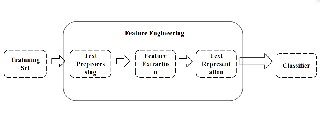
Figure 1. Process of Feature Engineering.

At present, text classification methods are gradually transitioning from traditional statistical and machine learning methods to deep learning methods based on complex neural network structures and are in a stage of rapid development. The use of deep learning methods for text classification has become a hot research pot in the current era, as it can effectively save costs and obtain information. In this field, computer scientists have developed neural networks, which are computational mathematical models that simulate biological neural networks[4]. The figure 2 presents the basic neuron model which constitutes the artificial neural networks. Artificial neural networks abstract the simulation of human brain neurons from the perspective of information and signal processing and simulate the connections between brain neurons by establishing multiple micro neuron models [5]. Its construction principle is to mimic the structure and composition of biological neural networks, established through the connections between a large number of neurons and neural synapses. This model can perform deep learning and analysis on text data, thereby achieving more accurate and efficient text classification. The use of text classification for data processing will have a broader application prospect.

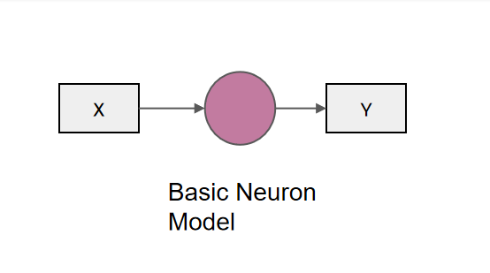
Figure 2. Basic Neuron Model.

The development of artificial neural network models originated from simple neural models[6], where each perceptron is a simple binary linear classification model. The perceptron processes input data through linear transformation and has a structure similar to biological neurons, including activated and inactive states. Neural networks can be seen as complex network models composed of an amount of perceptron. By connecting multiple perceptron to form different neural network structures, Neural networks can flexibly handle various complex problems. In neural networks, each perceptron is a basic neural unit with attributes such as input, weight, and activation function. By adjusting the connection weight values between neurons, neural networks can learn and adapt to different input modes, thereby achieving tasks such as classification and recognition of input data. In summary, perceptron is the foundation of neural network models, while neural networks are complex models composed of an amount of perceptron which are represented in the figure 3. By adjusting the connection weights and using different activation functions, neural networks can process and learn various input data. The figure 4 shows the basis model of feedforward neural network where the signal propagates one-way from the input layer to the output layer.

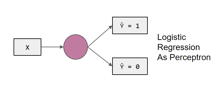
Figure 3. Perceptron.

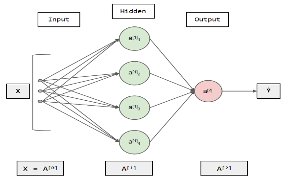
Figure 4. Feedforward Neural Network.

In recent years, with the increasing demand for massive text data analysis and the development and innovation of deep learning and neural network structures, text classification technology based on neural networks has become a key technology. This article will introduce the application and development process of neural network models with different structures in text classification, and compare their classification performance on text datasets to understand their advantages and disadvantages in processing text classification tasks. The figure 5 shows the deep neural network model which has multiple hidden layers.

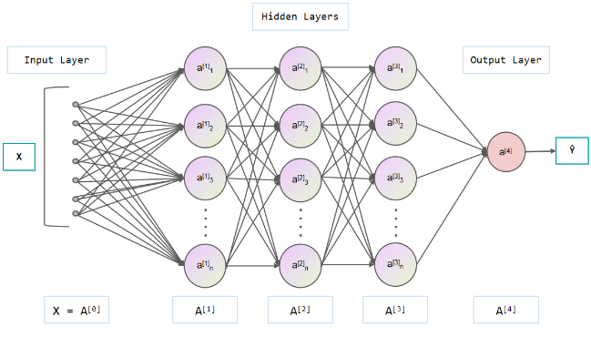
Figure 5. Deep Neural Network.

This article will introduce the application and development process of these neural network models with different structures in text classification and compare their classification performance on text datasets. By comparing the performance of these different structures of neural networks in text classification tasks, their performance and applicability can be evaluated. This article aims to explore the use of neural network models, long short-term memory[7] (LSTM), recurrent neural network[8] (RNN), and gated recurrent unit (GRU) to predict room occupancy and achieve more efficient room information resource management[9].

1.3. Paper Structure Overview

This article takes the text classification task as the background and studies the application of several neural network models with different structures in this task [10]. The article is divided into four chapters, each with specific research content. The main research content of each chapter is as follows:

Chapter 1 Introduction: Introducing the research background and significance of the text classification topic, as well as the current research status of text classification.

Chapter 2 Neural network model: This chapter provides a detailed introduction to the concept of neural network and several common model structures, including recurrent neural network, long short-term memory, and gated recurrent unit. The concepts, principles, structures, and characteristics of each model are explained and discussed.

Chapter 3 Experiment: The chapter describes the experimental environment and process, including the parameter configuration and explanation of related concepts used in the experiment, providing a basis for subsequent experimental results. This chapter also presents the experimental results and provides a detailed analysis and discussion of the experimental results. By comparing the classification performance of different neural network models on text datasets, some meaningful conclusions have been drawn.

Chapter 4 Conclusion: A summary of the entire experiment was provided, summarizing the main findings and conclusions of the experiment, and proposing some possible improvements and future research directions.

Through this article, we can learn about the application of neural networks in text classification tasks, and understand the characteristics and performance of different models. This has important reference value for further research and application of neural networks in the field of text processing.

2. Neural Network Model

2.1. Recurrent Neural Network

2.1.1. Recurrent Neural Network Conception. Human thinking has continuity and consistency when thinking. For example, when people communicate with each other, people can clearly remember what they said before and continue what they want to say next based on what they said before. However, it will become very difficult for most people to ask people to start with what they just said, push backwards, recall and deduce what they said before and say it. This shows that human thinking needs to rely on previous memory for thinking and reasoning. However, traditional neural network cannot achieve the continuity of memory. The traditional neural network is a feedforward network[11], each input is processed independently, and there is no memory or context information transfer. This leads to some problems in processing sequence data, such as information omission. In order to improve the traditional neural network, researchers have proposed recurrent neural networks. Recurrent neural network (RNN) introduces memory unit mechanism [12], which makes the network have memory ability and is shown in figure 6. The hidden state of RNN can capture the previous information and transmit it to the next state, so as to realize the memory and transmission of information.

2.1.2. Recurrent Neural Network Structure

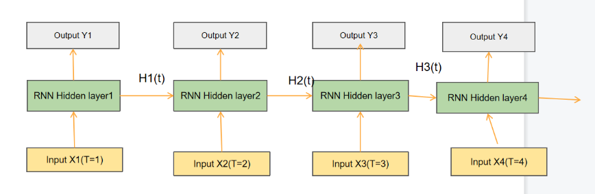
Figure 6. Structure of RNN.

Within recurrent neural network[13], the input and previous hidden state are combined into a new tensor, which is then processed through an activation function to generate a new memory state and shown in the figure 7. The recurrent neural network generally uses tanh () as the activation function. The function of this activation function is to help adjust the size of the value, so that the output value is within the interval (-1,1), thereby regulating the output of the neural network.

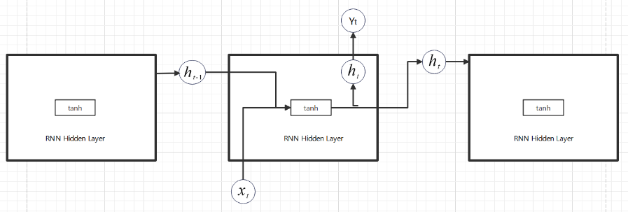
Figure 7. RNN Cell.

\( {h_{t}}=tanh({W_{hx}}{X_{t}}+{W_{hh}}{h_{t-1}}+{b_{h}})… \) (1)

\( {Y_{t}}=f({W_{0}}{h_{t}}+{b_{y}})… \) (2)

The specific internal propagation process can be expressed as follows: firstly, the input and the previous hidden state will be combined into a new tensor [14]. Then, this tensor will pass through the activation function to generate a new hidden state. Next, this new hidden state will be transmitted to the next cell, and then combined with the new input to form a new tensor, repeating the above steps.

Through this internal propagation process, recurrent neural network can remember information in sequence text data and use it for modeling. Recurrent neural network can effectively process sequence data through the combination of input and hidden states, as well as the role of activation functions and internal propagation processes, and have strong predictive abilities [15].

In recurrent neural network, the commonly used activation function is tanh () or relu(). The activation function can enhance the ability of the network and make the network better deal with complex data. Recurrent neural network has some problems when processing sequence data. One of them is short-term memory flaw, also known as long-term dependence problem. When the sequence data are long enough, it is difficult for recurrent neural network to transfer information memory from the early state to the later state, leading to the easy omission of important information memory.

Another issue is the disappearance or explosion of gradient during back propagation. Gradient vanishing refers to the phenomenon where the gradient value drops too small, resulting in the network being unable to effectively learn and train. The gradient explosion is caused by the excessive growth of gradient values, resulting in rapid updates of network parameters and inability to converge to appropriate values.

These issues will all affect the training and learning process of recurrent neural network because recurrent neural network has a long and continuous process of information transmission. Although recurrent neural network have issues such as short-term memory deficits and gradient vanishing/exploding, its performance and effectiveness in processing sequence data can be improved through some improved models and mechanisms [8].

2.2. Long Short-Term Memory

2.2.1. Long Short-Term Memory Conception. In 1997, Hochreiter and Schmidhuber proposed the long short-term memory network [16]. Long short-term memory (LSTM) is a special type of neural networks. By introducing gating mechanism, long short-term memory effectively alleviates the short-term memory problem in traditional neural network.

As for the conceptual differences between LSTM and RNN, we can better understand the differences between them through analogy. Assuming that RNN is like a greedy pig in the yard, it will not be picky or choose whether it is faced with delicacies or leftovers. The pig just wants to eat as much food as possible like recurrent neural network just wants to absorb as much information as possible. In contrast, LSTM is like an exquisite person. This person will not easily accept unhealthy and terrible food. He will carefully select healthy and balanced food which meet his taste and needs, and use tableware that meets his identity and taste because he has the right of choice and the ability of independent decision-making. The reason for this difference lies in the different design concepts and functional characteristics of them. Recurrent neural network is a simple recurrent structure, which has strong information storage ability and memory ability, but lacks the ability to filter and select information.

Therefore, Recurrent neural network will store all received information and process it without distinction. Long short-term memory will selectively store information, because it has strong ability. It has a gating device, and it can choose as much as it wants. The figure 8 shows the cell of long short-term memory. In short, LSTM is more flexible, efficient and accurate than RNN. By introducing gating mechanism and optimizing structure, LSTM can achieve better performance in different tasks.

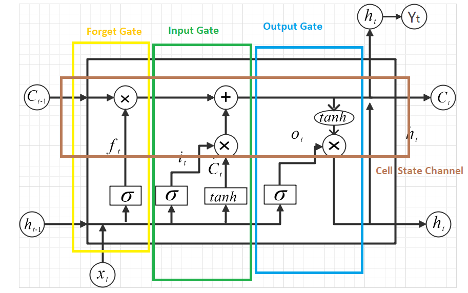
Figure 8. Lstm Cell.

2.2.2. Long Short-Term Memory Structure. Long short-term memory is a powerful neural network model, which introduces gating structure to control the addition or deletion of information in the cell state [10]. This gating structure is composed of an activation function and point multiplication operation. Specifically, LSTM mainly includes the following parts[7].

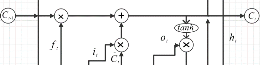
Figure 9. Structure of Lstm’s Cell State Channel.

\( {C_{t}}={f_{t}}×{C_{t-1}}+{i_{t}}×InputGate{C_{t}}… \) (3)

The first is the cell state channel, which includes two linear operations is shown in the figure 9. The first linear operation is used to control the proportion of the previous cell information, and the second linear operation is used to increase the new information brought by the input. The results of these two linear operations will be used to update the cell state. We multiply the tensor generated by the previous forget gate and the tensor with main cell state transmitted by the previous cell, and then add the tensor generated by the input gate to obtain the new tensor. Cell state channel is responsible for transmitting and preserving information during the whole process. It controls the flow and preservation of information through the adjustment of these gates.

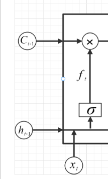
Figure 10. Structure of Forget Gate.

\( {f_{t}}=σ({W_{f}}{h_{t-1}}+{W_{f}}{X_{t}}+{b_{f}})… \) (4)

The second is the forget gate, which outputs a value between 0 and 1 based on the previous hidden state and the current input and is shown in the figure 10. If the output value is 0, it means to completely forget the historical information transmitted before; If the output value is 1, it means to completely retain the history information passed in before. The existence of forget gate can help neural network avoid redundancy and confusion of information. In long short-term memory, forget gate is an important part. Its role is to decide whether to retain or discard the previously learned information. When some information in the neural network is excited by sigmoid() activation function, its output value will be in the range of (0,1). Therefore, the existence of forget gate can help neural network better learn and adapt to different input data. By reasonably setting the activation function, the effect of neural network can be improved.

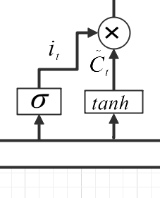
Figure 11. Structure of Input Gate.

\( {i_{t}}=σ({W_{i}}×{h_{t-1}}+{W_{i}}{X_{t}}+{b_{i}})… \) (5)

\( InputGate{C_{t}}=tanh{(}{W_{C}}\cdot {h_{t-1}}+{W_{C}}{x_{t}}+{b_{C}})… \) (6)

The third part is the input gate[7], which also outputs two information based on the previous hidden state and the current input: one represents how much information is added, and the other represents the strength of the information. This information will be used to update the cell status. The input gate controls the input of new information and determines which information should be added to the cell state channel. The figure 11 shows structure of Input gate.

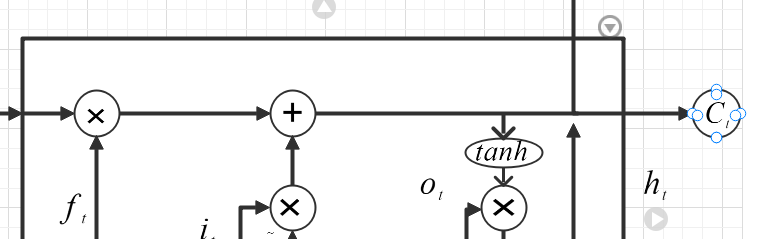
Figure 12. Structure of Update Gate.

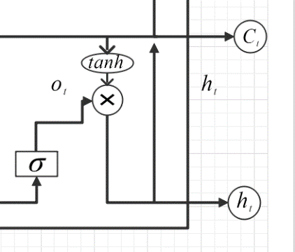
Figure 13. Structure of Output Gate.

The fourth part is the update gate, which outputs the next cell state based on the previous cell state, forget gate, input gate and new information. The Update gate is shown in the figure 12. The existence of this gating structure can help neural networks learn and reason more efficiently.

\( {o_{t}}=σ({W_{o}}{h_{t-1}}+{W_{o}}{x_{t}}+{b_{o}}). \) (7)

\( {h_{t}}={o_{t}}*tanh{(}{C_{t}})... \) (8)

The last part is the output gate, which adds an output gate based on the cell state of the update gate output to control how much information is output as a layer of the next state. The existence of this part can help the neural network to deal with different task requirements more flexibly. The figure 13 shows structure of Output gate. The basic structure of long short-term memory is composed of input gate, forget gate, output gate, update gate and cell state channel. These key components control the input, retention, output and transmission of information through different mechanisms, so that the long short-term memory network can effectively process sequential data and alleviate the long-term dependence and gradient problem.

2.3. Gated Recurrent Unit

2.3.1. Gated Recurrent Unit Conception. Gated recurrent unit is a variant of long short-term memory[9], which was proposed in 2014. Gated recurrent unit is very similar to long short-term memory. It discards the cell state of long short-term memory and uses hidden state to pass information. The figure 14 illustrates the basis cell of gated recurrent unit.

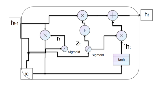
Figure 14. GRU Cell.

Gated recurrent unit is a simplified version of long short-term memory and has simpler structure than LSTM [9]. Gated recurrent unit, like LSTM, utilizes gating mechanisms, it can effectively control the flow of tensor, so that the network can better capture the long-term dependencies information. Gated recurrent unit further optimizes the cell structure composed of four gates in LSTM into a cell structure composed of two gates. This improvement not only maintains the original advantages, but also reduces the complexity of the model and improves the training efficiency and speed. In addition to simplifying the structure of the model, GRU also makes fusion and other improvements to cell state of long short-term memory. These improvements enable GRU neural network to better use context information to process long sequence data, thus improving the performance of the model. In a word, gated recurrent unit, as an improved model based on LSTM, provides strong support for the application of deep learning in various fields.

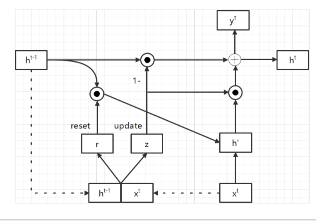
Figure 15. GRU Gating Mechanism.

Figure 16. GRU Gating Mechanism.

Gated recurrent unit consists of update door, reset door and hidden state.The structure of gated recurrent unit and special gating mechanism are presented in the figure 15 and figure 16.

2.3.2. Gated Recurrent Unit Structure. Gated recurrent unit is a simplified version of LSTM that has only two gates: reset gate and update gate [9]. The function of the update gate is similar to the input gate in LSTM. The update gate can decide which new tensor to add and control the transmission of new information. The reset gate is usually used to determine the degree of discarding previous information and control the elimination of old information. The two parts together constitute the basic structure of GRU model. Although there are some structural differences between GRU and LSTM. GRU does not have a cell state, while LSTM has a cell state. These differences enable GRU[9] to have higher computational efficiency in certain scenarios.The figure 17 illustrates the basis cell of gated recurrent unit.

\( {z_{t}}=σ({W_{u}}{h_{t-1}}+{W_{u}}{x_{t}}+{b_{u}}) \lt updategate \gt \) (9)

\( {r_{t}}=σ({W_{r}}{h_{t-1}}+{W_{r}}{x_{t}}+{b_{r}}) \lt resetgate \gt \) (10)

\( `{h_{t}}=tanh{(}W\cdot {r_{t}}*{h_{t-1}}+W\cdot {x_{t}}+{b_{h}}) \) (11)

\( {h_{t}}=(1-{z_{t}})*{h_{t-1}}+{z_{t}}*`{h_{t}} \) (12)

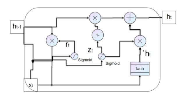
Figure 17. GRU Cell.

Due to structural differences, the number of parameters for GRU and LSTM also varies. GRU has fewer parameters, while LSTM involves more parameters. Therefore, in scenarios where computational resources need to be saved, GRU may be a better choice. There are also certain differences in training strategies between GRU and LSTM. Usually, using back propagation algorithm and Gradient Descent method can simultaneously optimize the parameters of GRU and LSTM. However, due to the relatively simple structure of GRU, special optimization techniques can sometimes be used to improve training effectiveness, such as using Momentum or Adaptive Learning Rate.

3. Experiment

3.1. Experimental procedure

3.1.1. Content. The relevant research in this article adopts the UCI (University of California Irvine) machine learning repository's room occupancy detection dataset, which is a set of text time series datasets that will be used to study the performance of neural network models in text classification tasks. The purpose of the study is to explore the role and performance of RNN[8], LSTM[6], and GRU in classification tasks on this text dataset by training them[9]. By comparing the experimental performance of these models in text data classification tasks and further studying the internal parameter structure of the models, it is expected to systematically discover the value of neural network models in deep learning in text classification tasks. For the experiment, I chose the room occupancy detection dataset provided by the UCI (University of California Irvine) machine learning repository. This dataset collected the properties of Light, Temperature, Humidity, Humidity Ratio, and CO2 in the room through experimental equipment and instruments to detect the occupancy of the room [17]. Through these experiments, we hope to gain a deeper understanding of the potential application of neural network models in text data classification tasks and provide reference and guidance for further research. The dataset’s attributes are presented in figure 18. Figure 18 shows the attribute information of the dataset.

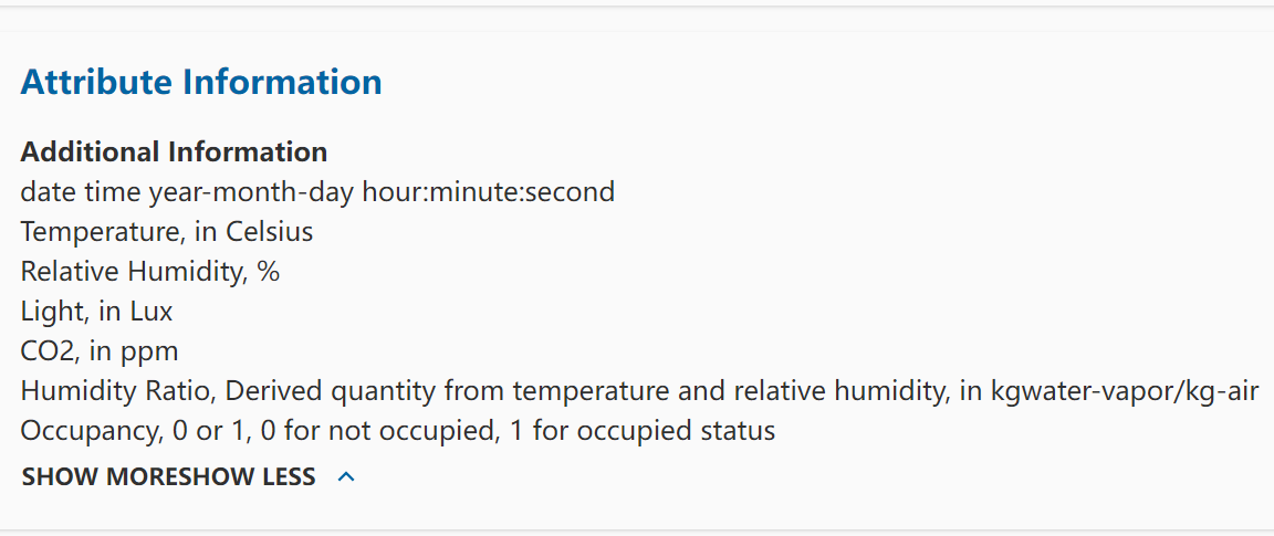
Figure 18. DataSet’s Attribute (Occupancy Detection DataSet on UCI Machine Learning Repository).

In terms of data preprocessing, I used Pycharm as the development environment and adopted Python version 3.7. To facilitate the installation and management of dependent toolkits, I used Conda and Pip as installation tools. In the data processing process, I used Numpy, a powerful library that can efficiently handle dimensional arrays and matrices. In order to solve the data analysis task, I chose Pandas, which is a tool based on Numpy and created to solve the data analysis task. I can use Numpy to store data more conveniently for subsequent data processing and analysis. In addition, in order to make the experimental dataset more intuitive and easy to understand, I also used Matplotlib for data visualization, in order to better display the experimental results. Through the application of these tools and technologies, data preprocessing and analysis can be carried out more efficiently and accurately, laying a solid foundation for subsequent experimental work. The figure 19 shows visualization of training set data and figure 20 shows visualization of test set data which are generated in the experiment through using the Matplotlib as the tool for data visualization.

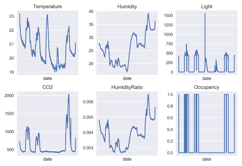
Figure 19. Visualization of training set data (0 for not occupied, 1 for occupied status) [Matplotlib].

By observing the line graphs of various values in the training set, it can be found that when the room is occupied, there will be significant fluctuations in temperature, humidity, light intensity, CO2 concentration, and humidity compared to these values. This indicates that the state of the room has a significant impact on these values, which further illustrates the correlation between the occupancy status of the room and these values.

In addition, it can be observed from the line graph of light intensity that there is an abnormally high light intensity at a certain time point. This may be due to errors in the data collection process of the photosensitive device, resulting in the presence of these noise points. It should be noted that these noise points may cause some interference to subsequent data analysis and model training, so it is necessary to pay attention to the handling of outliers when conducting data processing and model training. By observing the numerical line graph of the training set, it is possible to better understand the relationship between room occupancy status and various numerical values, and to conduct more accurate and effective data processing and analysis based on these characteristics in subsequent research to improve the performance and prediction accuracy of the model.

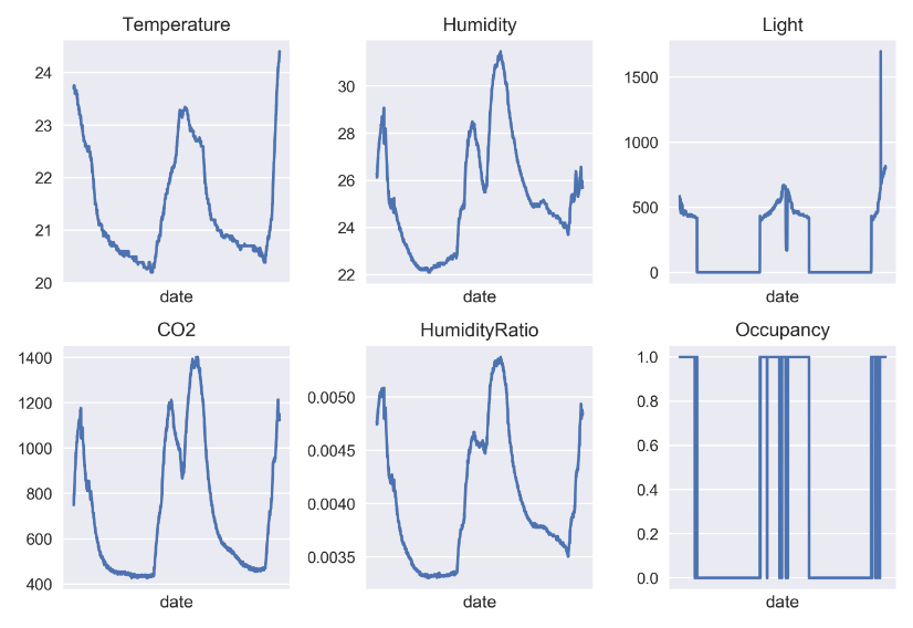
Figure 20. Visualization of test set data (0 for not occupied, 1 for occupied status) [Matplotlib].

According to the data from the test set, it is also shown that the temperature, humidity, light intensity, CO2 concentration, and humidity ratio values of the room will be significantly affected by the usage of the room, resulting in significant changes. This further validates the previously observed results of the training set. In different datasets, there is a correlation between room occupancy and values such as temperature, humidity, light intensity, CO2 concentration, and humidity ratio. This discovery is crucial for us to understand the relationship between room occupancy status and various numerical values, and these changes need to be considered in subsequent data processing and analysis. Only by fully understanding these influencing factors can we conduct more accurate data analysis and model training to improve the accuracy and performance of predictions.

3.1.2. Environment. Using my personal computer, the central processing unit(CPU) is Inter(R)Core(TM) I5-6300HQCPU@2.30GHz.The graphics processing unit(GPU) is NVDIA GeForce GTX960M. The computer’s ram size is 8G. In the experiment, I chose Pycharm as the integrated development environment and used Python 3.7 as the version of python. In order to build a neural network model, I used Pytorch, an open-source neural network library. Compared to Tensorflow, Pytorch adopts a dynamic graph structure, which means that Pytorch can create and generate networks at startup without the need to compile and run them first. This makes Pytorch more flexible and convenient in data parameter migration and debugging. To ensure the accuracy of the data, I preprocessed it. Considering the significant differences in the numerical distribution of various features, I used the StandardScaler class from the Sklearn library for standardization processing.

3.1.3. Configuration. In order to accurately predict the occupancy of a room, I designed an input layer with five input neurons, corresponding to five attributes: temperature, humidity, light, CO2 and humidity ratio. The values of these attributes will be used as inputs to the model to learn and predict the occupancy status of the room. In order to improve the expression ability and learning ability of the model, I constructed two hidden layers. Each layer contains 64 neurons. Through the connection and activation function of these neurons, the model can extract more abstract and useful features from the input data. Finally, I set up an output layer, which contains two neurons. These two neurons represent 0 and 1 of occupancy respectively, where 0 means the room is unoccupied and 1 means the room is occupied. Through the training model, I expect the trained neural network model can accurately predict the occupancy information state of the room. The basis structure of neural network model in the experiment is shown in the figure 21. Through the above analysis and design, I hope to get an efficient and accurate neural network model through training, which can be used to reliably predict the information of room occupancy.

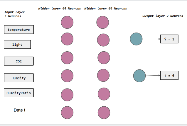
Figure 21. Experimental Structure of Basic Neural Network Model.

3.1.4. Concept. Optimizer: In the training process of neural network, optimizer is an important object, which updates the parameters of the model by calculating the gradient. In this experiment, I used an optimizer algorithm called Adaptive Moment Estimation Optimizer (Adam) and set the learning rate was 0.02. Adam algorithm is a random objective function optimization algorithm, which combines the idea of momentum and adaptive learning rate. Its design goal is to restrain the training loss of neural network without easily falling into the local optimal problem, and has high computational efficiency. By adaptively adjusting the learning rate, Adam can better adapt to the characteristics of different parameters, so as to improve the effect of training. The Adam optimizer shows good performance in the training process of neural network. It can not only restrain the training loss, but also maintain high computational efficiency. In practical applications, Adam optimizer is widely used and has achieved many good results. In the experiment, CrossEntropyLoss() was used as the loss function. Batch Normalization was also adopted, which normalizes each layer during the forward propagation of each batch of data. The concept of Normalization is shown in the figure 22.

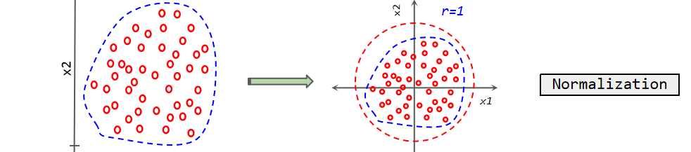
Figure 22. Normalization Concept.

Dropout: Dropout is an algorithm used to overcome the overfitting phenomenon of neural network. Its core idea is to train the network by shielding some neurons, and constantly change the shielded neurons during the training process. Specifically, dropout will shield some neurons before training, which can reduce the complexity of the network and avoid the problem of over fitting. Then, after updating the weight and other parameters through the back-propagation algorithm, dropout will restore the previously shielded neurons. Then, dropout will continue the next round of training and select a part of neurons at random again for shielding. By repeatedly shielding and restoring neurons, dropout can increase the robustness and generalization ability of the network. By using dropout, the trained network model can better adapt to the complex data and has better generalization ability. This is because dropout forces the network to learn more robust feature representation by randomly shielding neurons, rather than relying too much on some specific neurons. The figure 23 shows the concept of dropout.

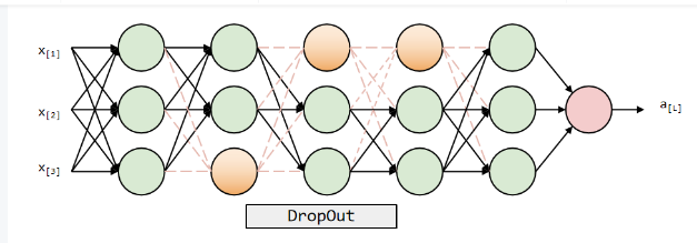
Figure 23. Dropout Concept.

Iteration: Iteration refers to the process of training a small dataset in batches. Typically, an epoch consists of multiple iterations.

Gradient: Gradient is a vector that points to the direction where the function's value rises the fastest. In back propagation algorithms, it often refers to the partial derivative of the error on the weight.

Gradient descent: Gradient descent is an optimization algorithm that updates parameters by calculating the gradient of the loss function under the current parameters. Its core idea is to achieve the optimal solution by continuously adjusting parameters to gradually reduce the loss function. Regardless of the type of machine learning and deep learning problem, gradient descent algorithm can be used to solve any objective function that needs to be optimized.

Stochastic gradient descent: Compared to other optimization algorithms, the stochastic gradient descent algorithm has many advantages. Firstly, it only uses the average of the gradients of a few non repeating sample points to update the model at a time, instead of using the average of the gradients of all sample points as traditional batch gradient descent algorithms do. This means that the stochastic gradient descent algorithm can greatly reduce computational complexity and thus improve efficiency. The stochastic gradient descent algorithm has the characteristic of fast convergence speed, so it is widely used in practical applications. The figure 24 shows differences between Batch Gradient Descent and SGD also illustrates differences of Batch Gradient Descent and Mini-batch Gradient Descent.

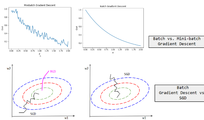
Figure 24. Differences Between Batch Gradient Descent and SGD.

Vanishing gradient problem: Vanishing gradient problem refers to the process of back propagation. Due to the chain derivative rule, if the value of this part is less than 1 when taking the partial derivative of the excitation function, the gradient update value will significantly decrease due to the increase in layers during the iteration process, and the weight update will be slow, resulting in the disappearance of the gradient.

Exploring gradient problem: Exploring gradient problem refers to the process of back propagation. Due to the chain derivative rule, when taking the partial derivative of the excitation function, if the value of this part is greater than 1, during the iteration process, as the number of layers increases, the gradient update value will significantly increase, and the weight update will be extremely fast, resulting in a gradient explosion.

Overfitting: Overfitting is a common problem in machine learning, referring to the phenomenon where a model performs well on the training set but poorly on the test set or new data. There are two main reasons for overfitting: firstly, the model is too complex, fitting the noise and outliers in the training set, resulting in the inability to generalize on new data; Secondly, the training set has a small sample size and cannot fully cover the entire data distribution. Overfitting can have a negative impact on the predictive and generalization abilities of the model. The concept of Overfitting is shown in the figure 25.

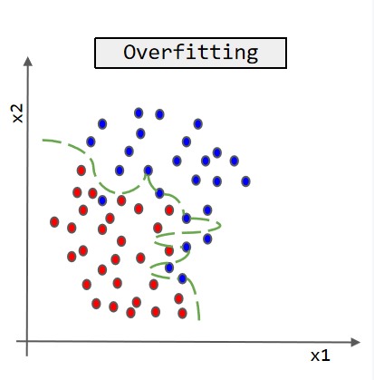
Figure 25. Concept of Overfitting.

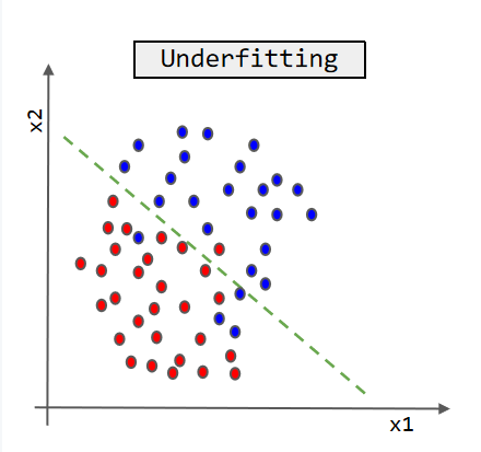
Figure 26. Concept of Underfitting.

Underfitting: Underfitting is an important concept in machine learning, which refers to the phenomenon where the model cannot fully fit the training data, resulting in a significant gap between the predicted results and the actual situation. The main reason for underfitting can be attributed to insufficient model complexity or insufficient training data. If the model is too simple to capture complex relationships in the data, it is prone to underfitting. In addition, if the training data volume is too small or the data quality is poor, it can also lead to the model not being able to learn the features of the data well. Underfitting has a significant impact on machine learning tasks. The figure 26 shows concept of Underfitting.

3.2. Recurrent Neural Network Result

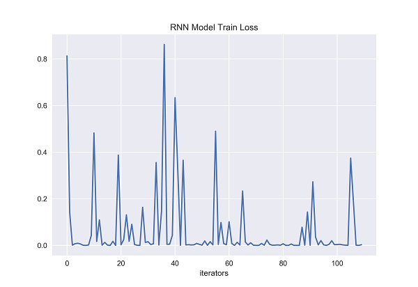
Figure 27. RNN Model Train Loss [Matplotlib].

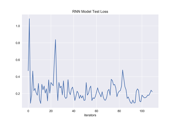
Figure 28. RNN Model Test Loss [Matplotlib].

The x-axis of both graphs represents the number of iterators that have been fed to the recurrent neural network. On the y-axis, the figure 27 represents the training loss of recurrent neural network, and the figure 28 represents the test loss of recurrent neural network. It can be clearly seen from the figure that the training loss of recurrent neural network fluctuates greatly when the number of iterators increases from 0 to 40. When the number of iterators reaches about 37, it rises sharply, and then drops sharply. It may be that such a situation occurs when encountering noise point data. With the increase of training time, the training loss fluctuates again when the number of iterators reaches about nearly 60 and then it remains relatively stable when the number of iterators is between 70 and 85. When the number of iterators reaches around 90 and 105, the training loss of recurrent neural network fluctuates again. It is obvious from the figure that the test loss of recurrent neural network fluctuates greatly with the increase of the number of iterators. Generally speaking, the test loss of RNN decreases with the increase of the number of iterators, but according to the whole test loss chart, the test loss of RNN has remained above 0.2 for most of the test time, and has a large fluctuation, which may be related to the data noise points, but it may also be that the RNN fitting degree is not good, or it may be related to the fact that the structure of the model itself can only remember the nearly information state.

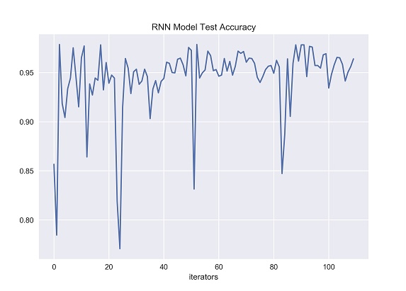
Figure 29. RNN Model Test Accuracy [Matplotlib].

The index value of the y-axis represents accuracy in the figure 29, which represents the classification accuracy obtained by using the test set in the recurrent neural network trained by the training set. The x-axis represents the number of iterators that have been fed to recurrent neural network.

According to the figure 29, with the increasing of the number of iterators, the prediction accuracy of recurrent neural network on the test set has changed very unstable. At some moments in the experiment, the accuracy of RNN even dropped below 0.90. During the test, when the number of iterators was close to 24, 50 and 83, the accuracy of recurrent neural network dropped greatly, from 20 to 24, and the accuracy dropped from nearly 95% to less than 80%, and then suddenly bounced back to the previous level. At the two points of 50 and 83, there was another sharp fluctuation and decline, and the overall trend was very unstable. According to the results of several experiments, the unstable reason may be that recurrent neural network has a special transfer structure, which can save the previous state and transfer state information to the subsequent state.

Recurrent neural network can only remember the state that is close to the current time, but it can not maintain the state information that is long before because recurrent neural network has the problem of short-term memory in design. Therefore, when the value of inputting data change greatly, the prediction accuracy of recurrent neural network is prone to be unstable. This is because recurrent neural network cannot effectively remember the state information of a long time ago, resulting in the limited processing ability of test set data with large fluctuations.

3.3. Long Short-Term Memory Result

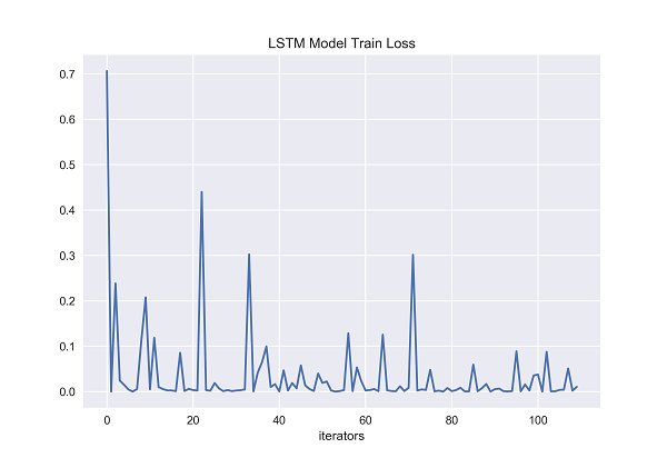
Figure 30. LSTM Model Train Loss [Matplotlib].

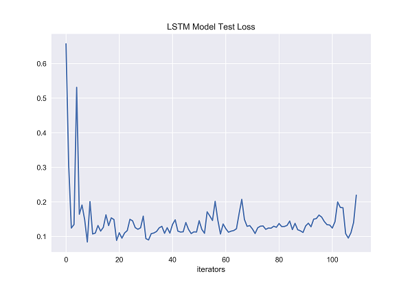
Figure 31. LSTM Model Test Loss [Matplotlib].

The x-axis of both graphs represents the number of iterators that have been fed to the neural network. On the y-axis, the figure 30 represents the training loss of long short-term memory, and the figure 31 represents the test loss of long short-term memory. The training loss of long short-term memory generally changes smoothly in most cases, but there are still significant changes when it encounters certain data, possibly due to data noise points, resulting in large changes. The training loss of long short-term memory does not exceed 0.1 in most cases. It can be seen that the model has been processed by gradient descent, and the error has been greatly reduced, indicating that the fitting degree of long short-term memory is good. It can be seen from the figure that with the growth of the test time, except for the initial period of time, the test loss of the long short-term memory generally remained between 0.1 and 0.2 during the whole test process, without much fluctuation, and the overall situation was relatively stable. The long short-term memory’s test loss has been shown to kept low level though the number of iterators is increasing. This result shows that long short-term memory can effectively reduce the loss while learning and adapting to test set data, and it can maintain good performance when faced with larger scale test data. This further demonstrates the superiority of long short-term memory when processing text-based time series data, as it can learn and capture long-term related information while maintaining a low loss during testing. Therefore, the gentle and consistently low level of variation in test loss on the long short-term memory further demonstrate its superior performance and stability in handling long text time-series data and related text classification tasks.

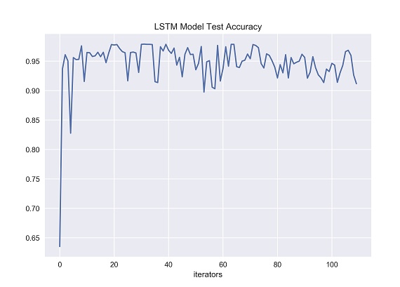
Figure 32. LSTM Model Test Set Accuracy [Matplotlib].

The index value of the y-axis represents accuracy, which represents the classification accuracy obtained by using the test set in the long short-term memory network trained by the training set. The x-axis represents the number of iterators that have been fed to the neural network. According to the figure 32, with the increasing of the number of iterators, the prediction accuracy of long short-term memory on the test set is generally stabled comparing recurrent neural network. It can be seen from the figure that the accuracy of LSTM remained almost stable above 0.95 for most of the entire experimental process. Long short-term memory is a variant of recurrent neural network, which contains three gate structures: forget gate, input gate and output gate. Through the control of these gates, long short-term memory can realize the long-term memory of valuable information, thus making up for the defect that recurrent neural network can only carry out short-term memory. Long short-term memory can learn and capture the long-term valuable information in time series data, so it has good performance in processing the classification task of time series text data. According to the results of many experiments, long short-term memory network can maintain a high level of prediction accuracy in the classification task of time series text data. Compared with the previous recurrent neural network, long short-term memory performs better in the stability of prediction and can better cope with the fluctuation of test data. In general, long short-term memory performs well in processing long time series text data, and has strong performance and stability. It is especially suitable for the classification task of time series text data.

3.4. Gated Recurrent Unit Result

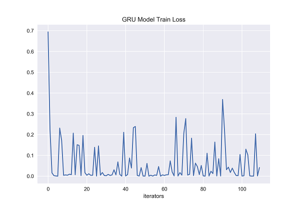
Figure 33. GRU Model Train Loss [Matplotlib].

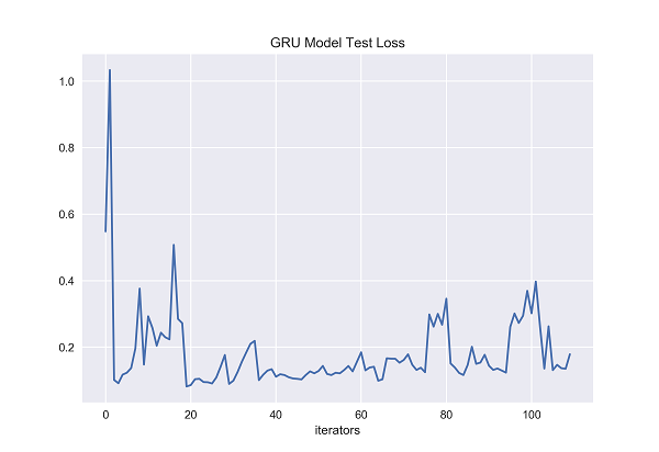
Figure 34. GRU Model Test Loss [Matplotlib].

The x-axis of both graphs represents the number of iterators fed to the gated recurrent unit. On the y-axis, the figure 33 represents the training loss of gated recurrent unit, and the figure 34 represents the test loss of gated recurrent unit. From the graph, it can be clearly seen that during the entire training period, gated recurrent unit's training loss fluctuates significantly compared to previous LSTM, and is very unstable. Even in the later stages of training, the loss value at a certain moment exceeds 0.3. Training loss of GRU is difficult to control below 0.1, while the training loss of previous LSTM was between 0 and 0.1 for most of the experiment, indicating that the training loss value of GRU is significantly higher than that of LSTM. During the entire testing period, compared to LSTM, GRU experienced significant fluctuations in testing losses and was unstable. The testing loss of GRU is not easily controlled below 0.2, sometimes exceeding 0.2 or even reaching 0.4 in the later stages of testing, which was not seen in previous LSTM testing losses. The previous LSTM testing loss was between 0.1 and 0.2 for most of the experimental time.

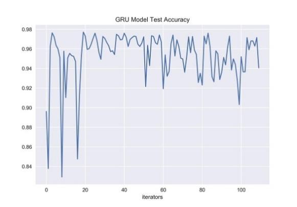
Figure 35. GRU Model Test Set Accuracy [Matplotlib].

The index value of the y-axis represents accuracy, which represents the classification accuracy obtained by using the test set in the gated recurrent unit trained by the training set. The x-axis represents the number of iterators that have been fed to the neural network. According to the figure 35, with the increasing of the number of iterators, gated recurrent unit's prediction accuracy on the test set becomes less stable. From the figure, it can be seen that although GRU maintained good accuracy according to the experiment, it was still very unstable. In the later stage of the experiment, the accuracy of GRU showed a significant decrease and then rebounded in the range of the number of iterators from 0 to 20 and 80 to 100, and even dropped to a level below 0.86 in the range of 0 to 20.

Although GRU, as a simplified version of LSTM, is efficient and time-saving in training neural networks, there are significant differences in prediction accuracy among neural networks trained multiple times. In contrast, LSTM performs better and more stably on time-series text data classification tasks. Through its internal gate structure, LSTM can effectively capture long-term information and keep long-term memory, resulting in better generalization performance when processing time series data. In summary, although GRU has efficient training performance, its overall generalization performance is not as stable and excellent as LSTM in time series text data classification tasks. Therefore, when selecting a neural network model suitable for processing time series data, LSTM is still a more reliable and effective choice.

4. Conclusion

This paper discusses the extensive application of neural networks in the field of data analysis and processing in deep learning, with a particular focus on text classification. When addressing the task of time series structured text data classification, this paper establishes three neural network models: recurrent neural network, long short-term memory and gated recurrent unit, and utilizes Pytorch deep learning library for experimentation. Though recurrent neural network has generally good performance in processing task of time series structured text data classification, experimental results show the trained recurrent neural network cannot maintain stability and high classification accuracy when processing some text data with long-term dependency information because of its short-term memory defects. The problem of short-term memory exists in the recurrent neural network, which means that the recurrent neural network can only remember the memory information of the previous period of time. When encountering long-time series of text data, the recurrent neural network cannot handle the problem of text data with long-term memory dependent information.

Long short-term memory performs best in the task of long time series structured text data classification, and has superior performance and stability. Because of its special structure, long short-term memory can selectively remember information, retain valuable information, transfer it to the next moment, and forget some meaningless information, which makes long short-term memory have more advantages than recurrent neural network in processing long-term serial text data. According to the experimental results, although gated recurrent unit can save a certain amount of training time compared with long short-term memory, its stability is slightly inferior to long short-term memory, and its effect is between long short-term memory and recurrent neural network. It is obvious that the network model trained based on long short-term memory has the best classification accuracy among the three neural network models. However, in practical problems, datasets are usually diverse and affected by external factors, and there are a large number of noise points. Therefore, it is crucial to further study and explore how to select appropriate methods to improve the generalization ability and maintain high classification accuracy of the model when dealing with the task of text data classification. Therefore, when facing other problems and solving these practical problems, experts and scholars still need to spend time together to explore and study in depth, in order to deal with diverse datasets and complex external factors.

References

[1]. Liu Hongpei Research on Chinese News Text Classification Based on Deep Learning [D]. Southwestern University of Finance and Economics, 2019.
[2]. Guo Hao Research and Implementation of a Text Emotion Analysis System Based on Neural Network Models [D]. Beijing University of Posts and Telecommunications, 2018.
[3]. Wan Qingling Text Analysis of Outbound Travel Commentary Based on Text-CNN and LSTM [D]. Zhongnan University of Economics and Law, 2020.
[4]. Wang Zhihui, Wang Xiaodong Research on Text Classification Methods Based on Neural Networks [J] Computer Engineering, 2020,46 (03): 11-17.
[5]. Cui Wei Analysis of the Factors Influencing Chinese Film Box Office and Production Level [D]. Jilin University of Finance and Economics, 2020.
[6]. Liu Ye Research on Hotel Intelligent Recommendation System Based on LSTM Model Analysis [D]. Shanghai Normal University, 2018.
[7]. Wu Juanjuan, Ren Shuai, Zhang Weigang, Wu Jing, Li Xiangyun A Daily Sales Forecast Method Based on LSTM Model [J] Computer Technology and Development, 2020,30 (02): 133-137.
[8]. Ding Peng Research on text classification and annotation of adverse drug reactions based on RNN [D]. Yunnan University, 2020.
[9]. Liu Yang Research on Time Series Prediction Based on GRU Neural Network [D]. Chengdu University of Technology, 2018.
[10]. Wang He Research on Financial Time Series Prediction Based on Text Analysis and LSTM [D]. Wuhan University of Technology, 2020.
[11]. Zhou Zhihua. Machine Learning [M]. Tsinghua University Press, 2016.
[12]. Wang Jingwen Empirical Analysis of Stock Prices Based on Recurrent Neural Networks [D]. Yunnan University, 2020.
[13]. Liu Yijiao Research on Stock Index Prediction Based on Trend Factor Preprocessing and Recurrent Neural Network [D]. Shandong University of Finance and Economics, 2019.
[14]. Zhang Yachao Research and Implementation of Text Classification Algorithms for Aerospace Intelligence [D]. Xidian University, 2019.
[15]. Chen Enhuan Multi scale Recurrent Neural Networks for Sequential Data Modeling [D]. South China University of Technology, 2020.
[16]. Hochreiter, S.,&Schmidhuber, J. (1997) Long short term memory Neural calculation, 9 (8), 1735-1780.
[17]. Accurate occupancy detection of an office room from light, temperature, humidity, and CO2 measurements using statistical learning models Luis M. Candanedo, V Ã © Ronique Feldheim Energy and Buildings Volume 112, 15 January 2016, Pages 28-39.
Cite this article
Zheng,M. (2024). Research on text classification based on neural networks. Applied and Computational Engineering,41,282-303.
Data availability
The datasets used and/or analyzed during the current study will be available from the authors upon reasonable request.
Disclaimer/Publisher's Note
The statements, opinions and data contained in all publications are solely those of the individual author(s) and contributor(s) and not of EWA Publishing and/or the editor(s). EWA Publishing and/or the editor(s) disclaim responsibility for any injury to people or property resulting from any ideas, methods, instructions or products referred to in the content.
About volume
Volume title: Proceedings of the 2023 International Conference on Machine Learning and Automation
© 2024 by the author(s). Licensee EWA Publishing, Oxford, UK. This article is an open access article distributed under the terms and
conditions of the Creative Commons Attribution (CC BY) license. Authors who
publish this series agree to the following terms:
1. Authors retain copyright and grant the series right of first publication with the work simultaneously licensed under a Creative Commons
Attribution License that allows others to share the work with an acknowledgment of the work's authorship and initial publication in this
series.
2. Authors are able to enter into separate, additional contractual arrangements for the non-exclusive distribution of the series's published
version of the work (e.g., post it to an institutional repository or publish it in a book), with an acknowledgment of its initial
publication in this series.
3. Authors are permitted and encouraged to post their work online (e.g., in institutional repositories or on their website) prior to and
during the submission process, as it can lead to productive exchanges, as well as earlier and greater citation of published work (See
Open access policy for details).