1. Introduction

The rapid advancement of information technology and growing frequency of user interactions are causing the Internet to generate massive amounts of data daily. This explosion of data, often referred to as "information overload," is not only putting significant load pressure on Internet infrastructure but also making it increasingly challenging for users and businesses to find relevant information efficiently.

Recommendation systems have emerged as a vital solution to the problem of information overload. These systems have become an integral part of daily life, guiding users through a sea of information based on their preferences. However, these systems face several challenges, including the "cold start" problem, where the lack of initial user data makes personalized recommendations difficult [1]. To address these challenges, the Multi-Armed Bandit (MAB) problem in reinforcement learning serves as a promising avenue for optimizing recommendation systems. Specifically, this study focuses on the efficacy of the Upper Confidence Bound (UCB) algorithm within the MAB framework. The LinUCB algorithm is a context-aware multi-armed bandit approach, designed to minimize cumulative regret through a balanced strategy of exploration and exploitation [2, 3]. It has been successfully implemented in Yahoo's personalized news recommendation system, significantly improving user engagement metrics such as clicks and read time. In summary, the LinUCB algorithm represents a significant advancement for recommendation systems. By leveraging user context, it can deliver highly personalized content, thereby enhancing user satisfaction and, consequently, the competitive advantage of various platforms. Cumulative regret serves as a measure of algorithmic performance, a concept that will be elaborated upon in subsequent sections of this study.

2. Problem Description

2.1. Multi arm slot machine problems and their basic concepts

2.1.1. Classical Multi-Armed Bandits. A learner and environment play a sequential game called a bandit problem (reflecting the uncertainly in decision-making and outcomes of the decisions). The game is performed on n tricks. In each rounds t=1,2,…,n, the learner chooses an action At from a set of k possible actions and receives a random reward Xt. The learner's aim is to maximize the cumulative reward over a period of time ,i.e., maximize \( \sum _{t=1}^{n}{X_{t}}={X_{1 }}+{X_{2}}+…+{X_{n}} \) .Then Regret =Reward lost by taking sub-optimal decisions(Largest possible cumulative reward in n rounds if we know which arm is the best) \( \sum _{t=1}^{n}{X_{t}} \) .It is crucial to balance the trade-off between exploration and exploration [4].

Figure 1 illustrates the model, highlighting how regret in reinforcement learning measures the performance gap between the learner's policy and the optimal policy within a set of competing policies [5]. This set of policies, often referred to as the competitor class Π, includes the optimal policy for all possible environments in E. By measuring the regret relative to Π, we can assess the learner's performance in terms of the loss incurred compared to the optimal policy. The regret captures the difference between the maximum expected reward achievable using any policy in Π and the expected reward collected by the learner. To ensure a comprehensive evaluation, it is important that Π encompasses the optimal policy for all environments in E. This way, the regret reflects the learner's performance relative to the best possible policy across all possible situations. The Environment does not reveal the reward of the action not selected by the learner. The learner should gain information by repeatedly selecting all actions which called exploration. When the learner select a “bad” action, it loses from the cumulative reward (The learner should try to “exploit” the action that returned the largest reward so far). Example: Two-armed slot machine, i.e., k=2, Let’s assume we played 10 rounds and receive the following rewards:

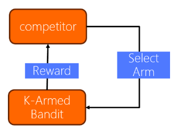
Figure 1. The relationship between the competitor and K-armed Bandit (Photo/Picture credit: Original).

Table 1. Action-Reward Distribution for Left and Right Moves Over 10 Trials.

Table 1. In the first 10 rounds, the left and right options were chosen five times each. Assuming 10 additional rounds to be played, the left option shows signs of improvement, boasting an average yield of $4, compared to the right option's average yield of $2. This situation illustrates one of the central challenges in bandit problems: the inherent uncertainty involved in selecting from multiple options. Suppose there are k arms l possible action: {1, …, k}. Reward from each action is a Bernoulli random variable, e.g.,

Reward from action I= \( \begin{cases} \begin{array}{c} 0, with probability 1-{μ_{i}} \\ 1, with probability {μ_{i}} \end{array} \end{cases} \) (1)

This k action can represent k different ads, and ui’s can be click probability of a user who is shown advertisement I. So, it is obvious to have E \( [Reward(i)]={μ_{i}} \) , i=1, …, k (expected value of the Reward from action I).

The muti-armed bandit problem is to sequeitially decide which action to take in each round 1, 2, …, n without any prior knowledge on the mean rewards \( {μ_{1 }},…, {μ_{k}} \) .if we know \( {μ_{i}} \) ’s, the optimal policy would be to take the action with the largest mean reward in all rounds, i.e.,

\( {k^{*}} \) =arg max \( {μ_{i}} \) , \( i∈\lbrace 1,…,k\rbrace \) (2)

And our total expected reward over n rounds with that choice would be n* \( {μ_{{k^{*}}}} \) The regret of any algorithm l policy is then given by the difference between n* \( {μ_{{k^{*}}}} \) and the total reward our policy has achieved, i.e.,

\( {R_{n}}=n*{μ_{{k^{*}}}}-E[\sum _{t=1}^{n}{X_{t}}] \) (3)

The regret in reinforcement learning is a measure of how much worse the learner's performance is compared to the best possible performance. It takes into account the randomness in the environment and the policy being used. The difference between the maximum expected reward achievable with any policy and the expected reward collected by the learner can be referred to as regret. The first term represents the best possible performance, while the second term represents the actual performance of the learner.

The regret depends on the specific environment and policy being used. In environments where the regret is large, it means that the learner is performing significantly worse than the best possible performance. On the other hand, in ideal cases, the regret would be small for all environments, indicating that the learner is performing close to the best possible performance. In all possible environments, the worst-case regret is the maximum regret that can occur. It represents the scenario where the learner performs the worst across all possible situations.

2.1.2. Types of Bandits Problems. Stochastic Stationary Bandits means that the Reward of each action comes from a fixed distribution [6]. None-Stationary Bandits explain that the Reward distribution may change over time. Structured Bandits means that There is a known “structure” in the way rewards from different arms are distributed. Then Contextual Bandits means before taking an action at each round, we receive a “side information” or “context” about the current state of the environment [7]. Over time the goal is to learn the best action for each context. The application of personalized recommendations, where the context can be user’s age | gender|.

Multi-armed gaming machine algorithms, as a form of reinforcement learning, discard the traditional reinforcement learning's characteristic of single-step forward, can be dynamically updated accordingly, and these dynamically updated parameters can continue to feed back to the system, thus realizing adaptive reinforcement Learning. Common multi-armed gaming machine algorithms in recommender systems include traditional MAB algorithms and MAB algorithms that take contextual information into account, among which traditional MAB algorithms include Thompson sampling, UCB algorithm (upward confidence interval block algorithm), Epsilon Greedy algorithm (greedy algorithm), LinUCB (linear upward confidence interval bounding algorithm), CBA (group UCB algorithm), Thompson sampling (Thompson sampling algorithm), Contextual MAB algorithms are commonly known as LinUCB algorithm.

2.2. Mathematical Model

In each round, an arm is selected and its associated reward is observed. If the kth arm is selected and a reward of x is obtained, the probability of receiving that specific reward can be calculated based on the probability distribution \( {r_{k}} \) . The objective is to maximize cumulative rewards through continuous arm selections, which requires a delicate balance between exploration and exploitation. In other words, the aim is not only to choose arms believed to yield high rewards but also to explore potentially high-rewarding arms by testing new options. A multi-armed slot machine, mathematically modeled with K arms, each featuring an unknown reward probability distribution, serves as the foundational framework for this problem [8]. The goal is to identify high-reward arms and maximize cumulative rewards by continually making selections. Various algorithms can address this challenge, enabling a trade-off between exploration and exploitation.

3. Overview of UCB algorithm principles

3.1. Basic ideas and working principles

To better understand their probability distributions, the algorithm prioritizes slots with higher upper confidence bounds for exploration. Slots with higher upper confidence bounds are prioritized by the algorithm for exploration to improve understanding of their probability distributions. The algorithm adjusts the upper confidence bound as exploration progresses and gradually opts to select slots with higher upper confidence bounds to use [9]. The maximum regret that can happen is the worst-case regret in any possible environment. In each round, assign a value to each arm (called the UCB index of that arm) based on the data observed so far that is an overestimate of its mean reward (with high probability), and then choose the arm with the largest value I index [10].

E.g.,

UC \( {B_{i}} \) (t-1) = \( \hat{{μ_{i}}} \) (t-1) +Exploration Bonus (4)

The item on the left is UCB index of arm I in round t-1, First item on the right is average reward from arm I till round t-1,then \( \hat{{μ_{i}}}(t-1)=\frac{\sum _{s=1}^{t-1}{X_{s}}1[{A_{s}}=i]}{{T_{i}}(t-1)} \) , Second item from the right is a decreasing function of \( {T_{i}}(t-1) \) which means number of samples obtained from arm I so far, so the fewer samples we have for an arm, the larger will be its exploration bonous. Being optimistic about the unknown supports exploration of different choices, particularly those that have not been selected many times. Should be large enough to ensure exploration but not so large that sub-optimal arms are explored unnecessarily .Let{ \( {X_{t}}, t=1,…,n \) }be a sequence of independent 1-subGaussian random variables with mean \( μ \) .Let’s \( \hat{μ}=\frac{\sum _{t=1}^{n}{X_{t}}}{n} \) ,then,

P ( \( \hat{μ}+\sqrt[]{\frac{2log⁡(\frac{1}{δ})}{n}} \gt μ \) ) \( ≥1-δ for all δ∈(0,1) \) (5)

The first term on the left-hand side of the inequality in parentheses is empirical average over n samples, the second term on the left-hand side of the inequality in parentheses is the term add to the average to over estimate the mean.

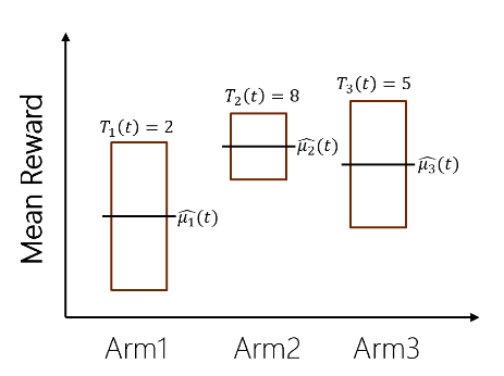
Figure 2. Average rewards of arm from their samples until round t (Photo/Picture credit: Original).

Figure 2 illustrates that the true mean rewards are likely to fall within the displayed confidence intervals. Notably, as the number of samples for an arm increases, the corresponding confidence interval becomes narrower. The best arm \( {i^{*}} \) to be selected many times so that:

\( {T_{{i^{*}}}}(t-1)→∞ and {\hat{{μ_{i}}}^{*}}→{μ_{{i^{*}}}} \) (6)

In other words the UCB index of the best arm will be approximately equal to its true mean \( {μ_{{i^{*}}}} \) .For all arms:

\( {UCB_{i}}(t-1)≥{μ_{i }}with high probability and recall that {μ_{{i^{*}}}}≥{μ_{i }} for all i≠{i^{*}} \) (7)

In a 2010 article published by scientists at UBC, the transformation of the UBC algorithm was explored for its application in Yahoo! News recommendations. This refined version of the UBC algorithm has been named LinUCB. A standout feature of LinUCB is its ability to incorporate relevant feature vectors into its calculations. LinUCB operates on the assumption that when an item is selected and presented to a user, the returns are linearly related to certain relevant features, often referred to as "context." These contextual features often form the most substantial part of the solution space in practical applications. Therefore, the experimental process involves predicting returns and confidence intervals based on user and item features. The item with the highest upper confidence bound is then recommended. Following this, observed returns are used to update the parameters of the linear relationship, thereby facilitating ongoing experimental learning.

3.2. Calculation method

At each round t=1, 2, …, n, choose the action:

\( {A_{t}}={arg_{i}} max {UCB_{i}} \) (t-1, \( δ \) )

\( ={arg_{i}} max⁡(\hat{{μ_{i}}}(t-1)+\sqrt[]{\frac{2log⁡(\frac{1}{δ})}{{T_{i}}(t-1)}}) \) (8)

where \( \hat{{μ_{i}}}(t-1) \) stands for average reward from arm I until round t-1, \( {T_{i}}(t-1) \) stands for number of times arm I is selected until round t-1.

3.3. Algorithm steps and processes

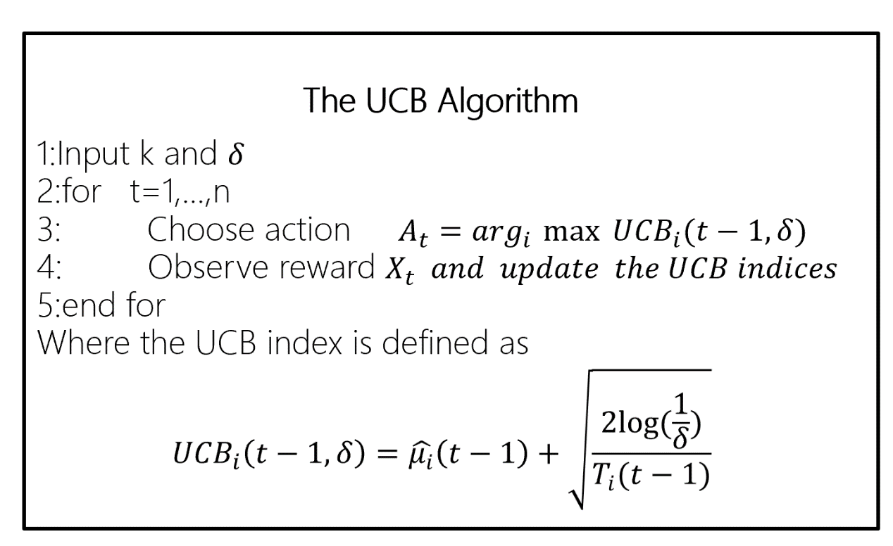
Figure 3. UCB Algorithm steps (Photo/Picture credit: Original).

Figure. 3. Shows that the process of the UCB algorithm. First, Calculate the average reward for each arm based on the historical data. Second, Calculate the upper confidence bound for each arm using the following formula: UCB = average reward + c * sqrt (ln(total number of rounds) / number of times the arm has been pulled), where c is a constant that determines the level of exploration. Third, Select the arm with the highest UCB value and pull it. Forth, Update the historical data with the new reward obtained from pulling the selected arm. Fifth, Repeat steps 1-4 until a certain stopping criterion is met.

4. Performance Analysis of UCB Algorithm

4.1. Theoretical analysis

The regret upper bound and the convergence speed constitute the theoretical analysis of the performance of the UCB algorithm. In this case, regret refers to the difference in average reward from the optimal arm during the computation. The convergence speed refers to the growth rate of the average reward in the near-optimal arm. The speed of convergence is evaluated by the number of choices.

4.2. Numerical experiments

It is significant to compare the performance of three multi-armed bandit (MAB) algorithms on real datasets, the MovieLens dataset is a vast collection of Movielens movie user reviews, which is commonly used in recommendation systems for algorithmic testing. The Grouplens team cleaned the data to remove user ratings that had less than 20 ratings or without complete demographic information.1,000,209 anonymous ratings of approximately 3,900 movies by 6,040 users who joined MovieLens in 2000.

Thus, to check their validity in real-world experiments, It is significant to run a sufficient number of experiments and look at the average value of the cumulative regret. Choose the horizon as n = 50, 000. For each algorithm run ten experiments and record the cumulative regret at each round t = 1, . . . , n in all experiments. For the ETC algorithm, set the length m*k of the exploration phase as \( ≅10\% of n,i.e., m*k≅5000. \) For the UCB algorithm, set the UCB index for arm I at round t-1 as

\( {UCB_{i}}(t-1)=\hat{{μ_{i}}}(t-1)+\frac{B}{2}\sqrt[]{\frac{4logn}{{T_{i}}(t-1)}} \) (9)

Where B is the difference between the maximum possible reward value and the minimum possible reward value. For example, for the Movie Lens dataset where rewards (i.e., ratings) can be in the interval 1-5 (stars), B should be set as 4. In general, a bounded random variable with difference between maximum and minimum value being B is σ-subgaussian where σ = B 2, and the exploration bonus needs to be updated as in. For the TS algorithm, updating the distributions \( {F_{i}}(t),i=1,…,k for \) the belief on the mean rewards of arms as following:

\( {F_{i}}(t)~Ν(\hat{{μ_{i}}}(t),\frac{\frac{{B^{2}}}{4}}{{T_{i}}(t)}), t=k+1,… \) (10)

where \( \hat{{μ_{i}}}(t) \) is the average reward of arm i until round t, B is as given above for the UCB algorithm, \( {T_{i}}(t) \) is the number of samples received from arm i until round t, and N (µ, σ2) stands for the Gaussian distribution with mean µ and variance \( {σ^{2}} \) .

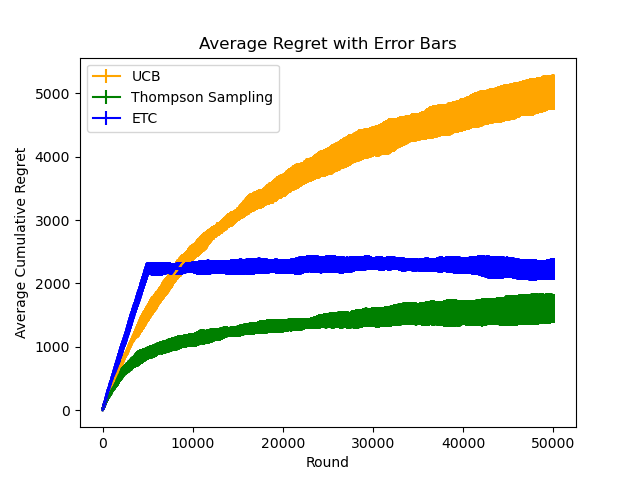
Figure 4. Average Regret with Error Bars (Photo/Picture credit: Original).

The theoretical findings introduced in lectures, such as the logarithmic scaling of cumulative regret for the algorithms discussed, hold true in the limit as n→∞. As shown in Figure 4. However, the actual size of n required to observe this logarithmic behavior may vary depending on specific circumstances, including the chosen algorithm and the underlying reward distributions.Set five different values for the horizon: n = 500, n = 5, 000, n = 50, 000, n = 500, 000, and n = 5, 000, 000. For the ETC algorithm, set the length m ∗ k of the exploration phase as 10% of n.

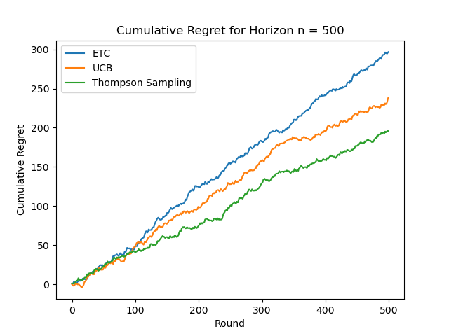
Figure 5. Cumulative Regret for Horizon n=500 (Photo/Picture credit: Original).

From the figure 5, it can be seen that the slope of ETC is higher, UCB is in the middle, and TS is lower. As n increases, TS shows logarithmic regret behavior and the gap between the three algorithms is clearly reflected, as shown in Figure. 6. At this time, ETC shows logarithmic regret behavior, as shown in Figure. 7. When n=500000, ETC has the largest cumulative regret value, forming a gap with the other two algorithms, and the cumulative logarithmic behavior of UCB is more obvious, as shown in Figure. 8. When n=5000000, the cumulative regret behavior of UCB is not obvious as shown in figure.9.

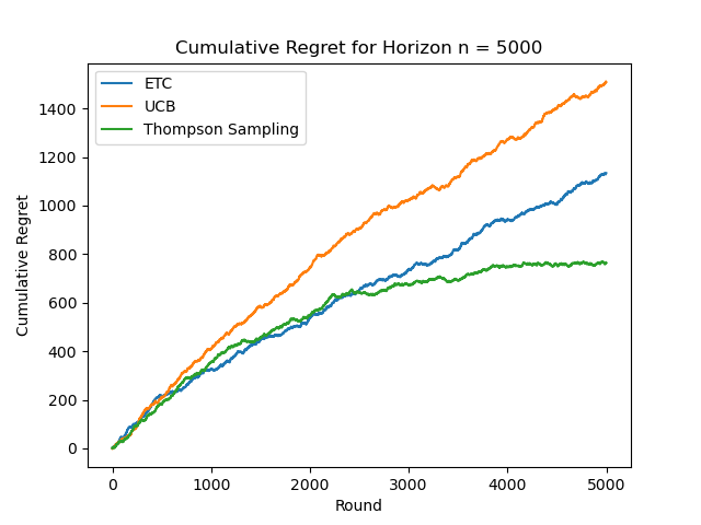
Figure 6. Cumulative Regret for Horizon n=5000 (Photo/Picture credit: Original).

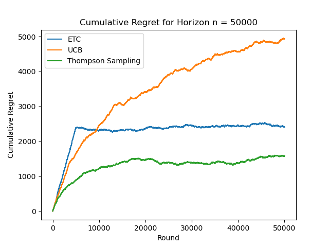
Figure 7. Cumulative Regret for Horizon n=50000 (Photo/Picture credit: Original).

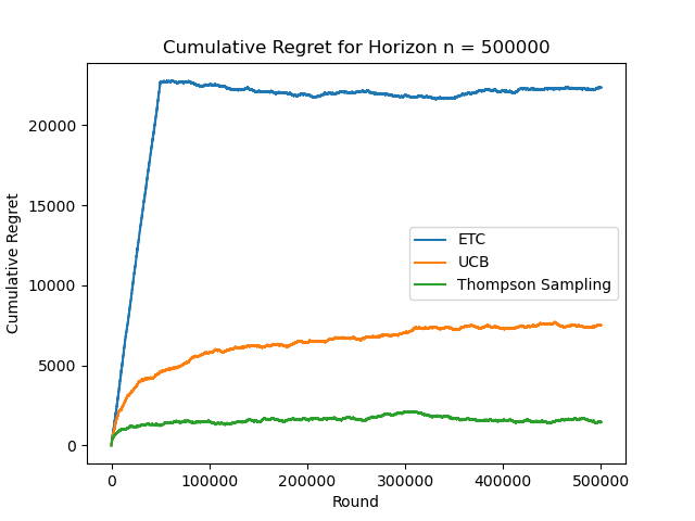
Figure 8. Cumulative Regret for Horizon n=500000 (Photo/Picture credit: Original).

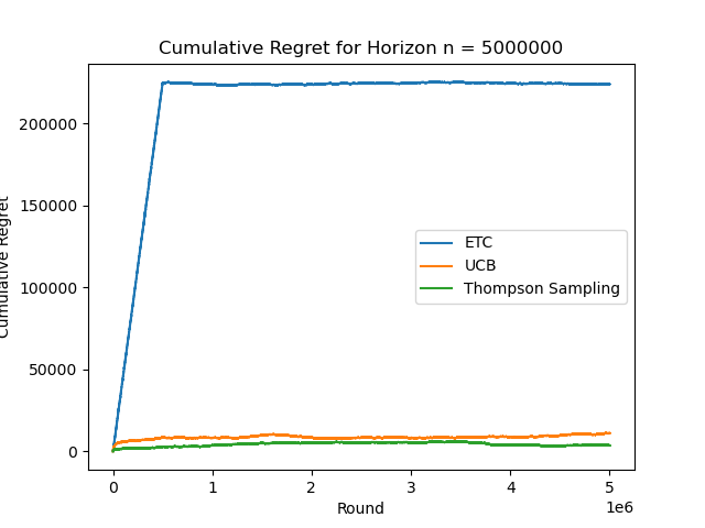
Figure 9. Cumulative Regret for Horizon n=5000000 (Photo/Picture credit: Original).

At n=5000, TS shows logarithmic regret behavior and at n=50000, UCB shows logarithmic regret behavior, this value varies from one algorithm to another. In order to compare the performance of the UCB and the asymptotically optimal UCB algorithms. It is significant to explore the impact of the exploration bonus on the algorithm performance. Choose n = 50, 000. The asymptotically optimal UCB algorithm uses the UCB index given as

\( {UCB_{i}}(t-1)=\hat{{μ_{i}}}(t-1)+B\sqrt[]{\frac{2log⁡(ƒ(t))}{{T_{i}}(t-1)}} \) (9)

Where \( ƒ(t)=1+t{(log{t})^{2}} \) . It is significant to compare the performance of the asymptotically optimal UCB and the standard UCB with three different \( τ \) values: \( τ \) = 1, \( τ \) = 2, and \( τ \) = 4. Note that, the larger is the \( τ \) value the more will the algorithm explore, while with smaller \( τ \) it will more aggressively exploit.

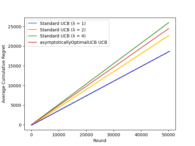
Figure 10. Comparison of Standard UCB and asymptotically optimal UCB (Photo/Picture credit: Original).

From the figure 10, it can be seen that as n grows, the overall rate of growth of cumulative regret value decreases, Standard UCB (lota=1) cumulative regret value is less than Standard UCB (lota=2), Standard UCB (lota=2) cumulative regret value is less than Optimal UCB, Optimal UCB cumulative regret value is less than Standard UCB (lota=4).

4.3. Algorithm Comparison

It is significant to set n = 1, 000, 000 and plot on the same figure the results for ETC, UCB, asymptotically optimal UCB, and Thompson Sampling algorithms (averaged over 100 experiments with error bars) and compare their performance.

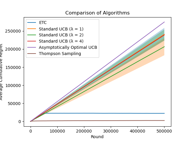
Figure 11. Algorithm Comparison (Photo/Picture credit: Original).

In the figure 11, Standard UCB (in=2), Standard UCB (in=4), and Asymptotically Optimal UCB go basically in the same direction, and Asymptotically Optimal UCB cumulative regret value is lower than that of Standard UCB, and the cumulative regret value of TS is shown to be the lowest as the round increases.

5. Application and Improvement Research of UCB Algorithm

The more accurate the extraction of user preferences is implied, the more effective the recommendation algorithm. The more efficient the recommendation algorithm is, the more precise the extraction of user preferences is implied. The extracting of item features with sufficient accuracy can also reflect the user's preference information to a certain extent. User preferences can be reflected by a lot of data generated about users and various information directly related to items. Labeled data related to users and projects is what we collectively refer to as labeled data, and we combine it to form multidimensional labels.

Initialisation: For each element, initialise its characteristic vector and covariance matrix. The algorithm's main concept is to use a linear model to model the user's preference and then use the upper bound confidence interval to select the optimal recommendation item.

The following are the specific descriptions:

First, for each element, initialize its functionality vector and its covariance matrix. Initiate the reward estimation and confidence interval for each item simultaneously. Second, Analyze the user's feature vector by analyzing their past behavior and feedback. Third, Using the current feature vector and covariance matrix, calculate the upper bound confidence interval for each item. The item's reward uncertainty range is represented by the upper confidence interval. Forth, Select the optimal item: according to the upper confidence interval, select the item with the largest upper confidence interval as the recommended item. Fifth, user feedback update: update the reward estimate and covariance matrix of the selected item based on user feedback. sixth, repeat steps 2-5 until a predetermined number of recommendations or convergence conditions are reached.

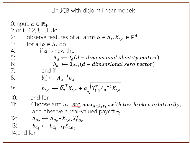
Figure 12. Algorithmic step (Photo/Picture credit: Original).

Figure. 12. Two advantages of the LinUCB algorithm can be summarized from the above process: The computational complexity is linearly related to the number of arms. Support dynamically changing candidate arm set.

The key to the LinUCB algorithm is the use of a linear model to model the user's preferences and to balance the strategies of exploration and exploitation by means of upper bound confidence intervals. By continuously updating the reward estimation and covariance matrix, the algorithm can progressively optimize the recommendation results and provide personalized recommendation suggestions.

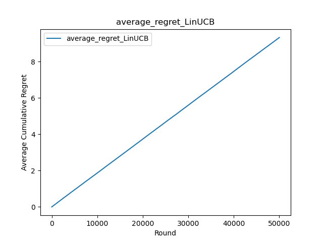
Figure 13. Average Cumulative Regret (Photo/Picture credit: Original).

Figure 14. Average Cumulative Regret (Photo/Picture credit: Original).

Figure 13 illustrates that cumulative regret values are linearly correlated. After multiple rounds of selection, these values reach single digits, optimizing the algorithm's performance in comparison to traditional UCB approaches. Figure 14 corroborates this, indicating that as the number of rounds increases, cumulative regret values maintain single digits without significant fluctuation. Summarizing the attributes of the LinUCB algorithm, several advantages come to the fore: Accelerated convergence relative to UCB algorithms is achieved through the inclusion of features, as substantiated in the paper. The effectiveness of the algorithm heavily hinges on feature construction, marking it as both a critical engineering challenge and an area of significant value. Due to the computational involvement of features, a dynamic pool of recommendation candidates can be managed, enabling editors to add or remove articles as needed.

Feature dimensionality reduction becomes essential for computational efficiency. When comparing LinUCB to traditional online learning models such as FTRL, two primary distinctions arise: LinUCB employs individual models for each arm, requiring the context to only encompass user-related and user-arm interaction features, thereby eliminating the need for arm-side features. In contrast, traditional online learning methods apply a unified model across entire business scenarios. Unlike traditional online learning models that employ a greedy strategy to maximize short-term gains without an exploration mechanism, LinUCB adopts a more effective Exploration and Exploitation (E&E) mechanism, prioritizing long-term overall benefits.

6. Conclusion

This study reveals that the cumulative regret value for LinUCB is in the single digits, indicating its distinct advantage in optimizing algorithms with a focus on long-term, overall benefits when compared to traditional UCB algorithms. This performance can be attributed to LinUCB's use of a linear model for modeling the reward function of each arm, allowing for a better fit in high-dimensional feature spaces. Such linear models facilitate more accurate reward predictions by learning the weights associated with each feature, thus providing a nuanced estimate of each arm's potential value. By employing a linear model, LinUCB adapts the reward function for each arm based on personalized user features. This enables the algorithm to deliver more tailored recommendations, which align closely with individual user preferences and characteristics. In contrast, traditional UCB algorithms assume a uniform reward function across all arms and are unable to offer personalized recommendations.

While LinUCB exhibits strong performance in multi-armed bandit problems, there exists scope for further refinement. Opportunities for future research include exploring avenues to enhance the algorithm's efficiency and accuracy. Although LinUCB employs a linear model for the reward function, some scenarios may involve more complex, nonlinear relationships. Investigating the application of nonlinear models to LinUCB could provide solutions for handling more intricate reward functions and contextual relationships.

References

[1]. Wang, M. (2021). Research on Algorithm Based on Cold Start Problem of Recommender System (Master's Thesis, University of Electronic Science and Technology of China).
[2]. Lai, T. L., & Robbins, H. (1985). Asymptotically efficient adaptive allocation rules. Advances in Applied Mathematics, 6(1), 4-22.
[3]. Yuan, M. (2019). Research on LinUCB recommendation algorithm based on multidimensional labels and user group characteristics (Master's thesis, Yanshan University).
[4]. Tang, L., Jiang, Y., Li, L., et al. (2015). Personalized recommendation via parameter-free contextual bandits. In Proceedings of the International ACM SIGIR Conference on Research & Development in Information Retrieval (pp. 323-332). Santiago, Chile.
[5]. Gong, X., Peng, P., Rong, L., Zheng, Y., & Jiang, J. (Year). Task analysis method based on deep reinforcement learning. Journal of System Simulation.
[6]. Zhao, X., Zhang, W., & Wang, J. (2013). Interactive collaborative filtering. In Proceedings of the 22nd ACM International Conference on Information & Knowledge Management (pp. 1411-1420). San Francisco, California, USA.
[7]. Khezeli, K., & Bitar, E. (2020). Safe linear stochastic bandits. Proceedings of the AAAI Conference on Artificial Intelligence, 34(06). https://doi.org/10.1609/aaai.v34i06.6581
[8]. Auer, P. (2002). Using confidence bounds for exploitation-exploration trade-offs. Journal of Machine Learning Research, 3(3), 397-422.
[9]. Huang, T. (2022). Application of multi-armed slot machine algorithm in federated learning client selection problem (Master's thesis, South China University of Technology).
[10]. Hu, Y., Liu, X., Li, S., & Yu, Y. (2021). Cascaded algorithm selection with extreme-region UCB bandit. IEEE Transactions on Pattern Analysis and Machine Intelligence.
Cite this article
Huang,R. (2024). Research on the principle, performance, and application of UCB algorithm in multi arm slot machine problems. Applied and Computational Engineering,47,1-13.
Data availability
The datasets used and/or analyzed during the current study will be available from the authors upon reasonable request.
Disclaimer/Publisher's Note
The statements, opinions and data contained in all publications are solely those of the individual author(s) and contributor(s) and not of EWA Publishing and/or the editor(s). EWA Publishing and/or the editor(s) disclaim responsibility for any injury to people or property resulting from any ideas, methods, instructions or products referred to in the content.
About volume
Volume title: Proceedings of the 4th International Conference on Signal Processing and Machine Learning
© 2024 by the author(s). Licensee EWA Publishing, Oxford, UK. This article is an open access article distributed under the terms and
conditions of the Creative Commons Attribution (CC BY) license. Authors who
publish this series agree to the following terms:
1. Authors retain copyright and grant the series right of first publication with the work simultaneously licensed under a Creative Commons
Attribution License that allows others to share the work with an acknowledgment of the work's authorship and initial publication in this
series.
2. Authors are able to enter into separate, additional contractual arrangements for the non-exclusive distribution of the series's published
version of the work (e.g., post it to an institutional repository or publish it in a book), with an acknowledgment of its initial
publication in this series.
3. Authors are permitted and encouraged to post their work online (e.g., in institutional repositories or on their website) prior to and
during the submission process, as it can lead to productive exchanges, as well as earlier and greater citation of published work (See
Open access policy for details).