


1. Introduction
Consumers can now better articulate their viewpoints and feelings about films due to the spread of online reviews and the development of social media platforms. Nevertheless, when confronted with multiple ratings and perspectives, individuals need help promptly and accurately grasping a movie's overall reputation and caliber. Consequently, movie sentiment analysis has become increasingly advantageous in aiding people to categorize and select films. This offers moviegoers a convenient guide to selecting films while providing essential data on audience feedback and industry trends for film production companies, marketing teams, and movie critics. As technology advances and research deepens, sentiment analysis in film will become increasingly important.
The examination of sentiment can be examined from various perspectives, including the document, sentence, and aspect levels [1]. This paper focuses specifically on the document view, classifying each review as positive or negative. Furthermore, the learning process can be supervised or unsupervised. Given that the IMDb review sentiment dataset chosen for this study is labeled, supervised machine learning is employed.
Neural networks are a computational model that simulates the human neural system. They comprise numerous artificial neurons and acquire knowledge by transmitting and linking information between neurons. Various problem-solving tasks, such as picture classification, audio recognition, and natural language processing, use neural networks. In recent years, the continuous improvement of computing power and the prevalence of big data have enabled neural networks to advance in various fields. They have become crucial tools in machine learning and artificial intelligence, offering robust modeling and predictive capacities for resolving intricate problems.
This article constructs a text classification model for sentiment analysis, which integrates machine learning models such as naïve Bayes, logistic regression, random forests, support vector machines, and deep neural network models utilizing encoder-decoder architectures. While text classification can be performed at the character level, our proposed model focuses on word-level learning [2].
There are four key sections to the article. A thorough analysis of the pertinent text classification literature is provided in Part II. Part III introduces the method employed in this research. The model's precise structure and the results of the experiments are presented in Part IV. Finally, Part V evaluates the findings and identifies upcoming difficulties.
2. Related works
This section of the manuscript provides a comprehensive assessment of the existing literature pertaining to the field of text classification.
In the early stages of machine learning technology, researchers primarily focused on feature extraction methods in sentiment analysis. Several papers provided overviews and comparisons of feature extraction methods, including those based on part-of-speech, statistical models, and dictionaries [3, 4]. Koto and Adriani conducted a comparative examination of nine feature sets in order to ascertain the most effective characteristics for sentiment analysis specifically on the Twitter platform, and found that methods such as AFINN and Senti-Strength were particularly effective [5, 6, 7]. Additionally, research in this field also involved the study of linguistic features and comprehensive evaluations of sentiment analysis tools [8, 9, 10, 11].
As artificial intelligence develops, deep learning techniques are being applied to sentiment analysis more and more. Various deep learning techniques have been utilized by researchers to tackle issues such as sentence-level sentiment analysis and aspect/object level analysis. These techniques include Convolutional Neural Networks (CNN), Recurrent Neural Networks (RNN), Long Short-Term Memory (LSTM) networks, Deep Neural Networks (DNN), and Deep Belief Networks (DBN) [12, 13]. They have also examined the merits, drawbacks, and performance metrics associated with each of these methods. Various applications of deep learning and machine learning methodologies have been explored, including aspect extraction and classification, opinion expression extraction, opinion holder extraction, irony analysis, and multi-modal data analysis [14]. Several researches suggest utilizing models such as sentiment-specific word embedding models, BERT, common sense knowledge, and cognition-based attention models to improve the effectiveness of sentiment analysis [15].
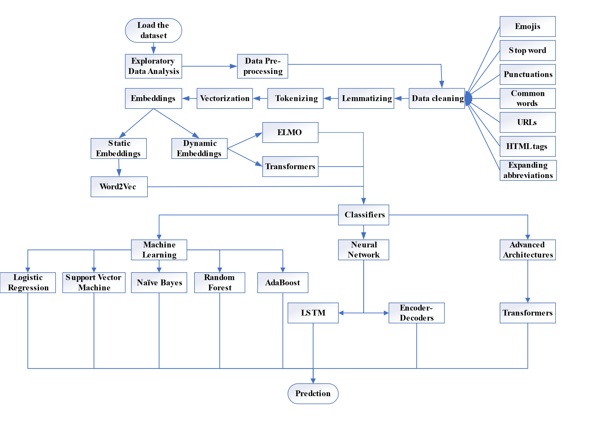
3. Proposed Methodology
In this part, a workflow of natural language processing (NLP) is proposed. Before the data is trained and fitted, the focus is on preparing the dataset, eliminating redundancies such as punctuation and stop words, and estimating the meaningfulness of the data.
All the steps are shown in Figure 1 as:
|
Figure 1. Global architecture of our classification system. |
3.1. IMDB dataset
The Internet Movie Database (IMDB) offers a substantial dataset comprising 50,000 movie reviews for the purpose of binary sentiment analysis. This dataset is evenly divided into two categories, with 25,000 reviews classified as positive and the remaining 25,000 reviews classified as negative. The regularly updated IMDB dataset can be viewed using the provided link. The Kaggle platform.
3.2. Exploratory data analysis
In this section, the conclusions presented are derived from the application of data visualization tools and syntactic analysis.
3.2.1. Conclusion 1. The dataset is balanced and contains equal number of semantics for reviews of both polarities.
3.2.2. Conclusion 2. The dataset contains redundant words and html syntaxes, punctuations and stop words are present in an equal distribution in the dataset.
3.2.3. Conclusion 3. This provides an outline as to the frequency of the conjunction of words which are occurring at the highest frequency. Another important aspect is that, there is a presence of certain html tags and punctuations which have to be removed as these are adding noise to the review corpus.
3.3. Data Preprocessing
3.3.1. Data cleaning. It removes unimportant words and elements (such as HTML tags, URLs, emojis, stop words, punctuations, expanding abbreviations, etc.) to retain only the most relevant words and ensure reliable results. And converting the labels to binary numeric which 1 for a positive rating, 0 for a negative rating.
3.3.2. Lemmatization. It makes the words be reduced to their root semantic word. Morphological transformations, such as converting "watched" and "watching" to their root form "watch", are performed through this technique. While stemming can be utilized, it is not recommended since it does not consider the semantics of the sentence or surrounding context. Stemming can also generate words not present in the vocabulary.
3.3.3. Tokenizing. The text is segmented into smaller entities or tokens in order to facilitate the quantification of word count and analysis of word frequency.
3.3.4. Vectorization. This enables conversion of the data into higher dimensional representations (matrices). These vectorization techniques transform the word corpus into a format amenable to more advanced semantic analysis. The implementation of vectorization without considering semantics involved the utilization of the TF-IDF approach.
TF-IDF: For the word \( i \) in \( j \)
\( {weight_{i,j}}={tf_{i,j}}×log{(\frac{N}{{df_{i}}}}) \)
\( {tf_{i,j}}=frequency with which i appears in j \)
\( {df_{i}}=sum of records that include the word i \)
\( N=total number of documents \) (1)
For retention of semantic importance, embedding is used instead.
3.3.5. Embeddings. The system employs pre-trained word vectors, assigning a probabilistic score to each word in the corpus. These probabilities are plotted in a low-dimensional space and word meanings are inferred from the vectors. Cosine distance is generally used as the primary metric to measure similarity between word and sentence vectors for inferring semantic similarity. Word Embeddings can either by static and dynamic.
Static word embeddings: These embeddings are pre-trained on large corpora such as Wikipedia, news corpora, etc.
Dynamic word embeddings: Deep contextual embeddings and sentence/word vectors are considered dynamic embeddings. These embeddings are deep contextual embeddings, meaning robust neural network models are needed for these architectures.
3.4. Classifiers
3.4.1. Machine Learning. 1). Logistic Regression (LR). The classifier known as logistic regression utilizes a sigmoid kernel throughout the training process. In supervised learning, Logistic Regression is a standardized model under generalized linear models that performs convex optimization by passing the cost function through the sigmoid kernel. The sigmoid function is defined by the following formulation:
\( S(x)=\frac{1}{1+{e^{-x}}} \) (2)
Because of its convergence properties and differentiability, the sigmoid kernel allows clamping of predicted values to binary labels.
2). Support Vector Machine (SVM). A popular supervised learning approach for classification and regression issues is the Support Vector Machine (SVM). Its core idea is to classify data by finding the optimal hyperplane in the feature space, which maximizes the distance between the closest samples from each class to the hyperplane. These closest samples are known as "support vectors" and are crucial elements of the decision boundary for an SVM classifier.
3). Naïve Bayes (NB). The Multinomial Naïve Bayes (MNB) model is a probabilistic classifier that use conditional probability to assign samples into categories or classes. It performs well with discrete integer-valued features like count vectors but can also be used with TF-IDF vectors. To determine conditional probability based on prior and posterior probabilities, MNB specifically employs Bayes' theorem.
\( P(forward eventbackword event)=\frac{P(backword event|forword event)P(forward event)}{P(backword event)} \) (3)
4). Random Forest (RF). The majority vote of the classes produced by the various trees is used to determine the predicted class in a random forest, which is a classifier made up of many decision trees.
5). Adaptive Boosting (AdaBoost). Adaboost, also known as Adaptive Boosting, is a widely utilized ensemble learning technique employed to improve the efficacy of weak classifiers. The fundamental concept of this approach is the iterative training of a sequence of weak classifiers, commonly referred to as base classifiers. Additionally, the sample weights are dynamically adjusted based on the performance of each individual base classifier. This ensures that in the subsequent training, more attention is given to the samples that were misclassified in the previous round, gradually improving the overall classifier performance.
3.4.2. Neural Network
1). Long Short-Term Memory (LSTM). The LSTM (Long Short-Term Memory) architecture is a type of recurrent neural network that is specifically designed to effectively address challenges associated with sequence data analysis. The utilization of this technique efficiently addresses the issue of long-term dependency in conventional Recurrent Neural Networks (RNNs), hence mitigating the problems of gradient vanishing or exploding. Consequently, it has found extensive applications in various domains such as speech recognition, natural language processing, machine translation, handwriting identification and other related subjects.
2). Encoder-Decoder (ED). Encoder-Decoder is a commonly used neural network architecture for handling sequence-to-sequence tasks such as machine translation and text summarization. The system comprises two primary elements: an encoder and a decoder, facilitating the transformation of input sequences with varying lengths into output sequences with varying lengths. This capability empowers the model to effectively process inputs and outputs of diverse durations.
3.4.3. Advanced Architecture
The Transformer model employs a self-attention method to effectively capture the interdependencies across various points within the input sequence, eliminating the necessity for recurrent or convolutional procedures. This allows Transformer to handle long sequences and perform parallel computations, leading to faster training speed and improved performance.
Due to hardware limitations of the experimental equipment, dynamic embedding and the use of transformer models were not implemented in this study.
4. Experimental Results
In the context of binary classification, the assessment of model performance entails the computation of performance measures derived from the confusion matrix, as presented in Table 1. In order to assess and compare the two models under consideration, the accuracy, which represents the percentage of correct predictions, is measured.
Table 1. Confusion matrix.
Result | Actual class | ||
+ | - | ||
Predicted | + | True Positive (TP) | False Positive (FP) |
- | False Negative (FN) | True Negative (TN) | |
\( Accuracy=\frac{TP+TN}{TP+TN+FP+FN} \) (4)
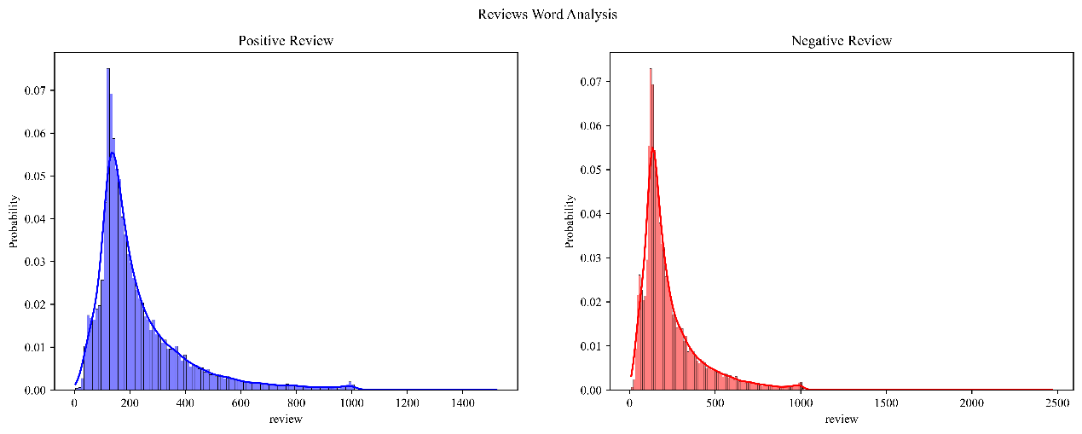
The distribution of the IMDB dataset movie reviews is displayed in figure 2.
|
Figure 2. Word Distribution of Movie Reviews |
The dataset was randomly divided into two parts with an 8 to 2 ratio, and the test set was employed as a validation set during model training.
Table 2. The split of dataset.
Dataset Type | Data volume |
Training | 40000 |
Validation | 10000 |
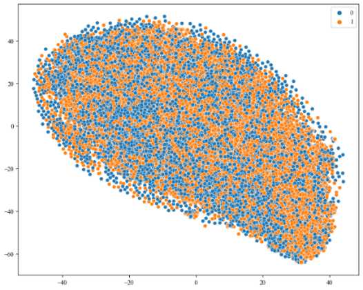
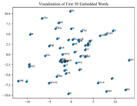
Figure 3(a) shows the vectorized reviews with TF-IDF, and figure 3(b) shows several words after embedding.
|
Figure 3. Vector space visualization. |
4.1. Machine learning models results
K-fold cross-validation was used for statistical models during training to improve result accuracy. The training set was segmented into 10 subsamples, with one subsample reserved for validation and the remaining 9 subsamples employed for training. K-fold cross-validation was repeated for each subsample, taking an average of the results across the 10 iterations or using alternative combinations, leading to an average training accuracy. The resulting trained model was applied to the validation set for category prediction, resulting in the accuracy of the validation set. Table 3 and Table 4 show the results of the training.
Table 3. Results of TF-IDF vectorized machine learning models.
Model (TF-IDF Vectorized) | Training Acc | Validation Acc |
LogisticRegression(max_iter=500) | 89.54% | 86.74% |
SVC(kernel='sigmoid') | 90.31% | 87.87% |
MultinomialNB() | / | 88.49% |
RandomForestClassifier() | 86.13% | 84.40% |
AdaBoostClassifier(learning_rate=0.01, n_estimators=100) | 67.15% | 68% |
Table 4. Results of Word2Vec embedded machine learning models.
Model (Word2Vec Embedded) | Training Acc | Validation Acc |
LogisticRegression(max_iter=500) | 62.79% | 61.81% |
SVC(kernel='sigmoid') | 57.60% | 56.68% |
MultinomialNB() | / | / |
RandomForestClassifier() | 60.22% | 60.25% |
AdaBoostClassifier(learning_rate=0.01, n_estimators=100) | 57.71% | 57.98% |
After testing, it was discovered that the accuracy of the statistical model decreased when lexical embedding was utilized. This implies a requirement for hyper-parameter tuning, and as such, we need to identify more suitable parameters to improve the model's performance.
4.2. Neural Network Results
For the training of the neural network, 40,000 data points were utilized from the dataset, while the remaining 10,000 data points were reserved for testing. The hyperparameters were set according to the following table.
Table 5. Hyperparameters of neural network structure.
Hyper Parameter | Definition |
maxlen | maximum allowed length of input text string (in this case, 1000) |
max_features | a maximum of 5000 words for the dictionary |
embed_size | dimensions (fixed at 300) of word embedding vectors |
4.2.1. LSTM. Figure 4 shows the baseline model structure to compare with other neural networks.
Figure 4. Diagram of basic structure of LSTM network [1]. |
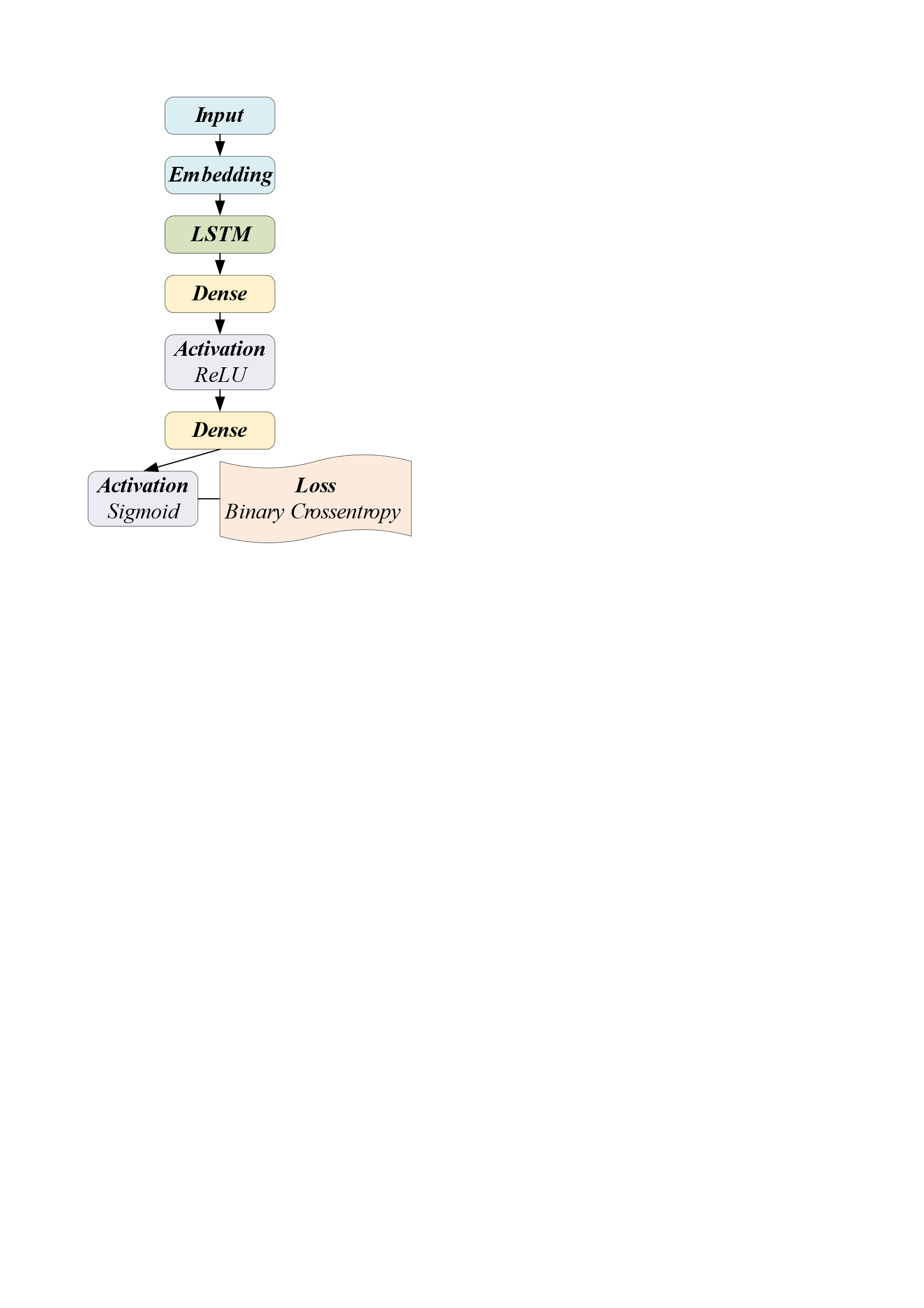
1). Embedding. The Embedding layer encodes the input integer sequences into dense vector representations, where each integer corresponds to a unique word. This layer transforms the input sequences into vector form.
2). LSTM. The LSTM layer specifies that it has 60 neurons. The LSTM layer takes the vector sequences obtained from the Embedding layer as input and extracts features by learning patterns and relationships within the sequences.
3). Dense. The fully connected layer (Dense) has 16 neurons and uses the ReLU activation function. This layer aids the model's acquisition of more complex feature representations. The output layer (Dense) has only one neuron and uses the sigmoid activation function. Since this text classification model is for a binary classification task, the output layer has one neuron, and the sigmoid function is used to convert the output value into a probability value between 0 and 1.
4). Loss function & Optimizer. It sets the loss function to binary cross-entropy, the optimizer to Adam, and specifies accuracy as the metric for evaluation.
|
| |
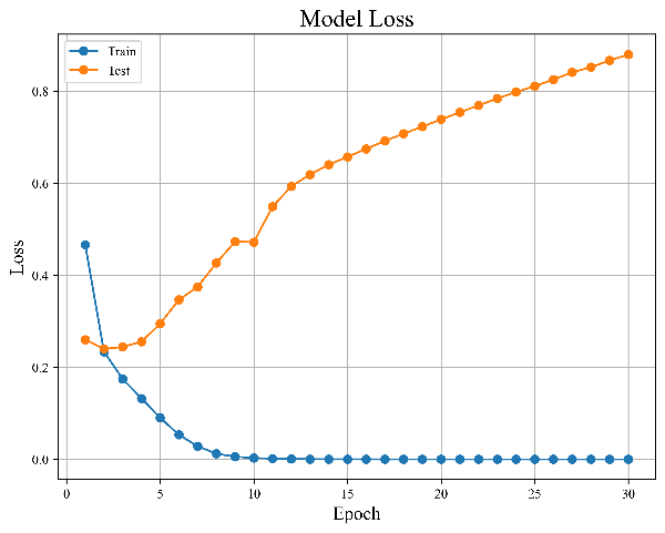
Figure 5. Results of baseline LSTM model | ||
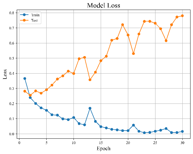
As illustrated above, Figure 5(a) and 5(b) display the model's error and accuracy distribution with the increase in the number of training sessions.
If pre-trained word sense embeddings are used, the model architecture is shown below.
|
Figure 6. Structure of bidirectional LSTM model [1]. |
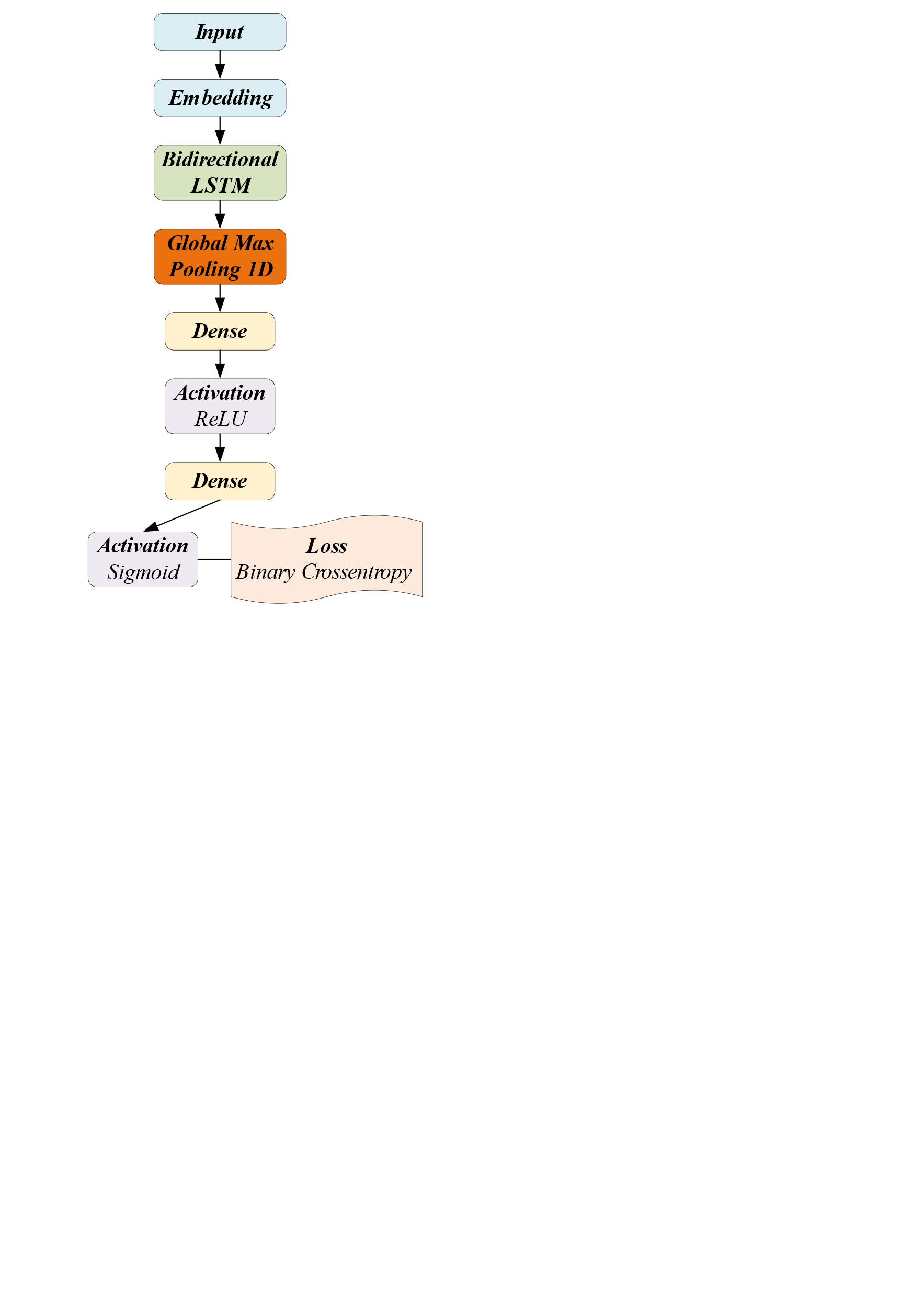
5). Bidirectional LSTM. Compared to a regular LSTM layer, the bidirectional layer has the property of considering contextual information from both past and future states, leading to more accurate predictions.
6). Global Max Pooling 1D. The GlobalMaxPool1D layer is a pooling layer used for dimensionality reduction. It performs element-wise maximum pooling along the time dimension of a sequence, converting a variable-length sequence into a fixed-length vector representation. The primary objective of this layer is to extract the crucial information from the sequence, without considering the specific time steps. Consequently, its impact is consistent across the whole sequence. The utilization of this particular layer is commonly observed in tasks involving sequence classification. Its purpose is to mitigate the computational difficulty of the model by diminishing the dimensionality of the output derived by LSTM or CNN layers.
|
| |
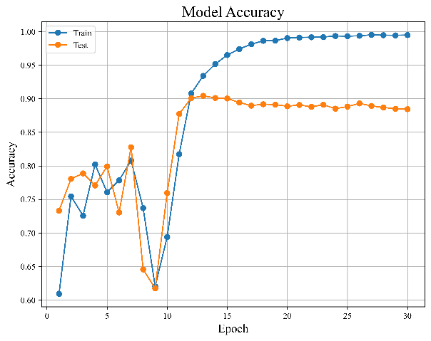
Figure 7. Results of bidirectional LSTM model | ||
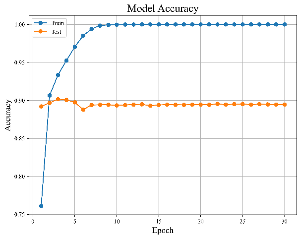
Figures 7(a) and 7(b), which are shown in the figure above, indicate how the distribution of the model's error and accuracy changes as the quantity of training sessions rises.
The pre-trained word vectors embedding_matrix from Word2Vec [16] is passed as weights in the Embedding layer of this model.
4.2.2. Encoder-Decoder (ED). Figure 8 shows the baseline model structure to compare with other encoder-decoders.
|
Figure 8. Structure of baseline ED architecture [1]. |
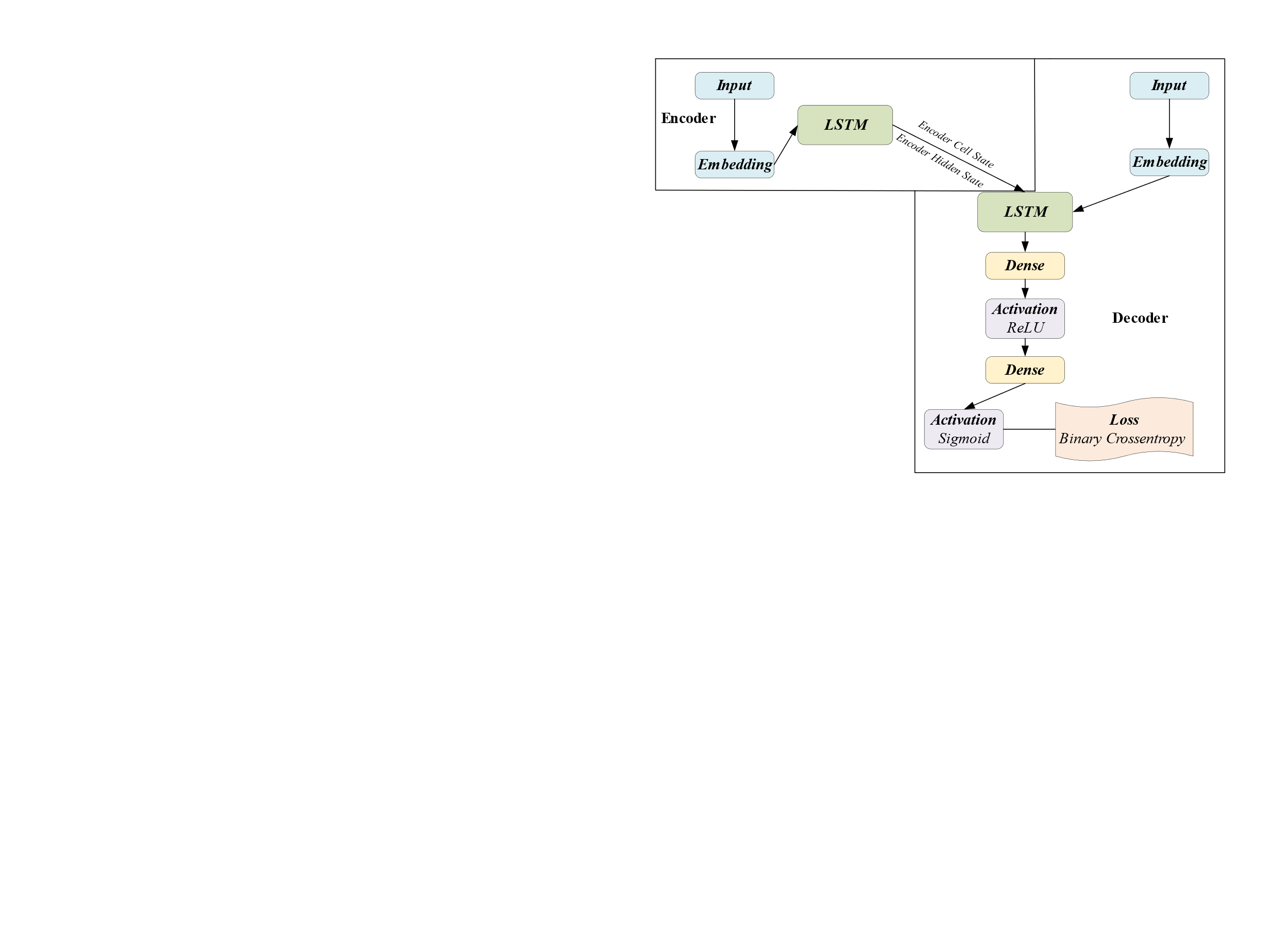
In order to provide the input sequence to the encoder, an input layer must first be built. The input sequence is then transformed into dense embedding vectors by the addition of an embedding layer. The embeddings will be updated during training because the trainable parameter is set to True.
The embedded input sequence is then processed by an LSTM layer with 60 LSTM units. This layer also returns the final hidden states (encoder_state_lstm_h) and cell states (encoder_state_lstm_c) of the LSTM in addition to the outputs.
For the decoder component, the same procedure is done. To process the target sequence, two layers are made: an input layer and an embedding layer. The max_features and embed_size used by the encoder are also used by the embedding layer.
The embedded target sequence is then processed after the addition of an LSTM layer. The initial state for the decoder LSTM is the initial state of the encoder LSTM, which consists of the final hidden state and cell state. This enables the decoder to consider the context that the encoder learned.
To transform the LSTM outputs, a dense layer with 16 hidden units and ReLU activation is applied. The final prediction is included as a dense layer with a single hidden unit and sigmoid activation.
Finally, utilizing the Model function and the encoder, decoder, and decoder output as inputs and outputs, the model is produced. An overview of the model's architecture is printed before it is returned.
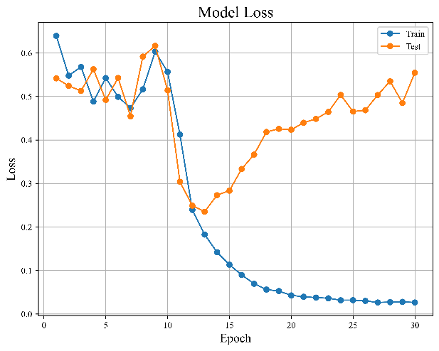
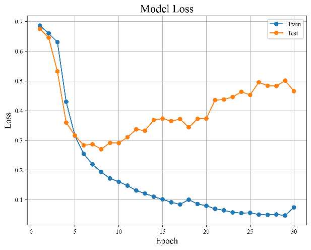
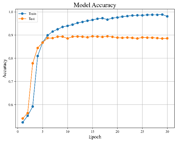
Figure 9(a) and 9(b) display the model's error and accuracy distribution with the increase in the number of training sessions.
|
| |
Figure 9. Results of baseline ED architecture. | ||
For the case of pre-trained word sense embeddings, the model architecture is shown below.
|
Figure 10. Structure of bidirectional LSTM ED architecture [1]. |
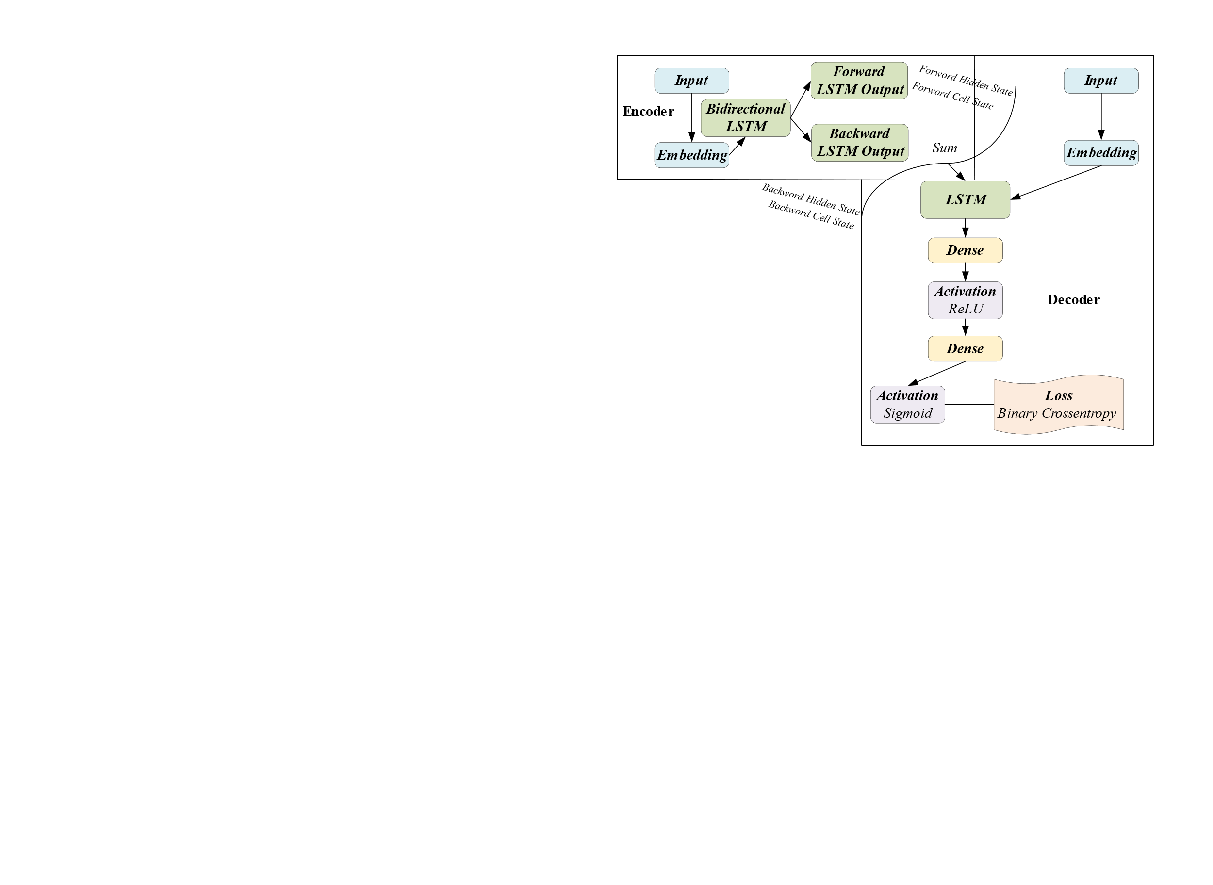
As opposed to before, the encoder has a bi-directional LSTM layer defined, which contains 60 LSTM cells and returns the output of the LSTM, as well as the final hidden state and cell state of the forward LSTM and the reverse LSTM. Utilizing the 'sum' operation, the outputs of the forward and reverse LSTMs are combined.
|
| |
Figure 11. Results of bidirectional LSTM ED architecture. | ||
5. Conclusion
Based on experiments, it was discovered that machine learning models show less adaptability to word sense embedding compared to neural networks. By repetitively and iteratively training the neural network model, a relatively high accuracy rate of 88% or above can be maintained.
However, it should be observed that the neural network model's error rate gradually rises with the number of training cycles, showing a propensity for overfitting in our model. Furthermore, during the initial training rounds, we observed that certain portions of the neural network model achieved an accuracy rate of over 90%. This indicates that in order to improve our model, we must either decrease the number of training rounds or optimize model hyperparameters. Furthermore, neither dynamic lexical embedding or transformer models were used in this investigation. Future research could look into how these models can be used to improve results.
References
[1]. Yenter A and Verma A 2017 2017 IEEE 8th Annual Ubiquitous Computing, Electronics and Mobile Communication Conf. (UEMCON) 540-546
[2]. Zhang X, Zhao J and LeCun Y 2015 Advances in Neural Information Processing Systems 28 649-658
[3]. Feldman R 2013 Communications of the ACM 56 4 82-9
[4]. Ahmad SR, Bakar AA and Yaakub MR 2019 Intelligent data analysis 23 1 159-89
[5]. Koto F and Adriani M 2015 Natural Language Processing and Information Systems 9103 453-457
[6]. Nielsen F A 2011 arXiv preprint arXiv 1103 2903
[7]. Thelwall M, Buckley K and Paltoglou G 2012 Journal of the American Society for Information Science and Technology 63 1 163-73
[8]. Taboada M 2016 Annual Review of Linguistics 2 325-75
[9]. Schouten K and Frasincar F 2015 IEEE transactions on knowledge and data engineering 28 3 813-30
[10]. Medhat W, Hassan A and Korashy H 2014 Ain Shams engineering journal 5 4 1093-113
[11]. Ravi K and Ravi V 2019 Knowledge-based systems 89 14-46
[12]. Prabha MI and Umarani Srikanth G 2019 2019 1st Int. Conf. on Innovations in Information and Communication Technology (ICIICT) 1-9
[13]. Ain QT, Ali M, Riaz A, Noureen A, Kamran M, Hayat B and Rehman A 2017 International Journal of Advanced Computer Science and Applications 8 6
[14]. Zhang L, Wang S and Liu B 2018 Wiley Interdisciplinary Reviews: Data Mining and Knowledge Discovery 8 4 e1253
[15]. Habimana O, Li Y, Li R, Gu X and Yu G Science China Information Sciences 63 1-36
[16]. Church KW 2017 Natural Language Engineering 23 1 155-62
Cite this article
Xia,S. (2024). Machine learning and deep learning-based sentiment analysis of IMDB user reviews. Applied and Computational Engineering,53,113-125.
Data availability
The datasets used and/or analyzed during the current study will be available from the authors upon reasonable request.
Disclaimer/Publisher's Note
The statements, opinions and data contained in all publications are solely those of the individual author(s) and contributor(s) and not of EWA Publishing and/or the editor(s). EWA Publishing and/or the editor(s) disclaim responsibility for any injury to people or property resulting from any ideas, methods, instructions or products referred to in the content.
About volume
Volume title: Proceedings of the 4th International Conference on Signal Processing and Machine Learning
© 2024 by the author(s). Licensee EWA Publishing, Oxford, UK. This article is an open access article distributed under the terms and
conditions of the Creative Commons Attribution (CC BY) license. Authors who
publish this series agree to the following terms:
1. Authors retain copyright and grant the series right of first publication with the work simultaneously licensed under a Creative Commons
Attribution License that allows others to share the work with an acknowledgment of the work's authorship and initial publication in this
series.
2. Authors are able to enter into separate, additional contractual arrangements for the non-exclusive distribution of the series's published
version of the work (e.g., post it to an institutional repository or publish it in a book), with an acknowledgment of its initial
publication in this series.
3. Authors are permitted and encouraged to post their work online (e.g., in institutional repositories or on their website) prior to and
during the submission process, as it can lead to productive exchanges, as well as earlier and greater citation of published work (See
Open access policy for details).
References
[1]. Yenter A and Verma A 2017 2017 IEEE 8th Annual Ubiquitous Computing, Electronics and Mobile Communication Conf. (UEMCON) 540-546
[2]. Zhang X, Zhao J and LeCun Y 2015 Advances in Neural Information Processing Systems 28 649-658
[3]. Feldman R 2013 Communications of the ACM 56 4 82-9
[4]. Ahmad SR, Bakar AA and Yaakub MR 2019 Intelligent data analysis 23 1 159-89
[5]. Koto F and Adriani M 2015 Natural Language Processing and Information Systems 9103 453-457
[6]. Nielsen F A 2011 arXiv preprint arXiv 1103 2903
[7]. Thelwall M, Buckley K and Paltoglou G 2012 Journal of the American Society for Information Science and Technology 63 1 163-73
[8]. Taboada M 2016 Annual Review of Linguistics 2 325-75
[9]. Schouten K and Frasincar F 2015 IEEE transactions on knowledge and data engineering 28 3 813-30
[10]. Medhat W, Hassan A and Korashy H 2014 Ain Shams engineering journal 5 4 1093-113
[11]. Ravi K and Ravi V 2019 Knowledge-based systems 89 14-46
[12]. Prabha MI and Umarani Srikanth G 2019 2019 1st Int. Conf. on Innovations in Information and Communication Technology (ICIICT) 1-9
[13]. Ain QT, Ali M, Riaz A, Noureen A, Kamran M, Hayat B and Rehman A 2017 International Journal of Advanced Computer Science and Applications 8 6
[14]. Zhang L, Wang S and Liu B 2018 Wiley Interdisciplinary Reviews: Data Mining and Knowledge Discovery 8 4 e1253
[15]. Habimana O, Li Y, Li R, Gu X and Yu G Science China Information Sciences 63 1-36
[16]. Church KW 2017 Natural Language Engineering 23 1 155-62