1. Introduction

Historically, the art and science of stock prediction have been an ever-evolving subject. As the stock market matures, its complexity increases along with more investors in the market. Consequently, factors affecting fluctuations in prices abound making the market seem more erratic. The effort to understand such a market and make predictions accordingly is a persistent force and inspired a plethora of research and experiments. Despite advancements in technologies and scientific methods, underlying theories remained in place, even with ongoing debates: the Efficient Market Hypothesis (EMH) and Adaptive Market Hypothesis (AMH) [1]. The EMH emerged in the mid-20th century, suggesting that stock prices reflect all available information, making consistent portfolio outperformance of the market challenging. However, market anomalies and behavioural biases led to critiques of EMH's all-encompassing efficiency. This paved the way for the AMH in the early 2000s, proposing that markets exhibit both rational and irrational behaviours, evolving over time. While EMH underscored the challenges of prediction, AMH highlighted the potential for adaptability and behavioural patterns in stock markets.

The most part of stock market forecasting history is about time series data. Most conventional models fall under the Generalized Autoregressive Conditional Heteroskedasticity (GARCH) family, including Auto-Regressive, Auto-regressive Moving Average, Auto-Regressive Integrated Moving Average [2]. The GARCH captures the changing volatility of price by modelling the variance of the current time based on past observations and past variances. With the advancement in technology, market forecasting methods evolved from simple technical analysis, identifying patterns through charts, to models that interpret data using algorithms, and finally to incorporate machine learning, as well as deep learning, to efficiently study a vast amount of data to find patterns. Nowadays, while recognizing the effect of sentiments on the stock market, new models that study sentiment analysis (SA) which analyses the influence of news and other information on investors become a trend [3].

Stock market forecasting emerges as a result meant for testing the understanding of the market. The significance of such predictions benefits both ways. It has conducive effects on both investors, individual and institutional investors, and the market itself. The interaction between total factor productivity (TFP) and stock prices indicates that a positive market shock could result in increased productivity [4]. While accurate predictions can lead to better portfolio management and risk assessment, an upward prediction that paints a positive picture of individual sectors of the stock market could boost consumer confidence and galvanize spending and investment, which consequently benefits the economy through increased productivity. Moreover, as research conducted in the Baltic stock market confirmed market inefficiencies [5], more factors were found that would undermine the EMH, like excess volatility, investor overreaction, seasonality in return, etc. If a forecasting model is built with machine learning that includes a vast amount of real-time news and information in its prediction, information asymmetry can be largely reduced, restore market fairness, curtail extreme price volatilities, and allow broad investors to trade rationally. As a result, the market can operate with higher efficiency.

In recent years, different forecasting models using different approaches have gained some impressive results. In 2020, Khan et al. used ARIMA(1,1,33) to forecast Netflix’s stock price from 2015 to 2020 [6]. The result yields that the measurement of Mean Absolute Percent Error indicates 99.75% accuracy and the prediction shows continuity in value in the next 100 days. In the same year, Xue et al. built a model using LSTM and compared it with a traditional Recurrent Neural Network(RNN), the Back Propagation(BP) neural network, and discovered that the LSTM yields high accuracy in forecasting stocks [7]. Apart from applying LSTM by itself, Wu et al. used a new method called Sequence Array Convolutional LSTM (SACLSTM), which used Convolutional Neural Network(CNN) to extract important features from historical data, options, and futures, along with traditional LSTM, to perform accurate prediction [8]. They compared results from models used and did not use this information and found that models with CNN-processed features yield lower accuracy loss. Another research subsidized the same preference for the CNN-LSTM model and compared it to Multilayer Perceptron(MLP), CNN, RNN, and LSTM CNN-RNN and found that CNN-LSTM resulted in the lowest Root Mean Squared Error(RMSE) and the highest R-squared among all [9]. In 2022, Abraham et al. used a genetic algorithm for feature engineering and employed random forest to forecast trends of 15 stocks and obtained 80% accuracy [10]. Moreover, as sentiment analysis gained more attention in forecasting models, Sonkiya et al. used Google’s pre-trained transformer model, BERT, to perform sentiment analysis on news and headlines of Apple Inc. and Generative Adversarial Network (GAN) to forecast the stock price. As a result, the proposed model (named S-GAN) outperformed other baseline models included in the experiment and exhibited early convergence because of the sentiment vector [11].

With the purpose of producing accurate forecasts of stock prices to gain profits from the market, this paper will delve into two popular models–the ARIMA model and LSTM model–to compare their forecasting performance on three stocks: APPL(Apple), AMZN(Amazon), and MSFT(Microsoft). This paper will compare the detailed steps of both methods and results obtained by testing trained models on the same dataset.

2. Data and method

The data used in experiments are the historical stock prices from September 1st, 2021 to September 29th, 2023 of the three stocks: APPL, MSFT, and AMZN, specifically focusing on their daily closing prices. To enhance the predictability and capture more stable trends inherent in stock price movements, this raw data is processed to compute the 5-day moving average for each stock. This methodology is aimed at mitigating the daily volatilities and noise, resulting in a smoother representation of the stock’s trajectory. The processed datasets were then chronologically partitioned into distinct subsets: training (60%), validation (20%), and test (20%) sets. This structure ensures an organized workflow where the model is trained on past data, its parameters are fine-tuned using the validation set, and finally, its performance is rigorously evaluated on the most recent data in the test set, providing a comprehensive assessment of its forecasting capabilities in real-world scenarios.

For the purpose of evaluating the accuracy of forecasting and compare the results of the two models, the root mean squared error (RMSE) and R-squared ( \( {R^{2}} \) ) are employed as criteria to evaluate performance. The RMSE calculation is shown below:

\( RMSE=\sqrt[]{\frac{1}{n}\sum _{i=1}^{n}{({y_{i}}-\hat{{y_{i}}})^{2}}} \) (1)

where n is the number of data points, \( {y_{i}} \) is the real value, and \( \hat{{y_{i}}} \) is the prediction. The closer the value of RMSE is to 0, the more accurate the prediction of the model because it perfectly aligns with the actual data without discrepancy. The \( {R^{2}} \) formula is shown below:

\( {R^{2}}=1-\frac{\sum _{i=1}^{n}{({y_{i}}-\hat{{y_{i}}})^{2}}}{\sum _{i=1}^{n}{({y_{i}}-\bar{{y_{i}}})^{2}}} \) (2)

where \( \bar{{y_{i}}} \) is the mean of the observed data. The closer \( {R^{2}} \) is to 1, the more data could be explained by the model, an indication of an effective model.

Table 1. Parameter Setting of LSTM.

LSTM is a type of recurrent neural network (RNN) architecture model proposed by Schmidhuber et al. in 1997 [12]. RNNs are neural networks that can recognize and remember patterns in sequences of data. However, vanilla RNNs have limitations, particularly when dealing with long-term dependencies because of the vanishing gradient problem. In other words, as sequences get longer, RNNs become unable to learn and carry information from earlier time steps to later ones. LSTM was introduced to address these limitations. LSTM’s memory cells contain three gates: input, forget, and output. Formulae for the three gates are as follows. The forget gate determines whether old information should be forgotten, in other words, assigning lower weights to it. The formula is shown below:

\( {f_{t}} = σ({W_{f}}\cdot [{h_{t-1}},{x_{t}}]+{b_{f}}) \) (3)

where \( σ \) represents the sigmoid function, \( {W_{f}} \) is the weight, \( {h_{t-1}} \) is the previous output, \( {x_{t}} \) is the input information, and \( {b_{f}} \) is the forget gate bias. The previous output and the current input are inputted into the input gate, and the output value and the potential cell state value are obtained:

\( {i_{t }}=σ({W_{i}}\cdot [{h_{t-1}},{x_{t}}]+{b_{i}}) \) (4)

\( {\widetilde{C}_{t}}=tanh{({W_{c}}\cdot [{h_{t-1}},{x_{t}}]+{b_{c}})} \) (5)

Here, \( {W_{i}} \) is the weight for the input gate and \( {W_{c}} \) is the weight for the cell state. \( {b_{c}} \) and \( {b_{i}} \) are biases. One updates the cell state according to the formula below:

\( {C_{t}}={f_{t}}*{C_{t-1}}+{i_{t}}*{\widetilde{C}_{t}} \) (6)

The previous output, \( {h_{t-1}} \) , and the input, \( {x_{t}} \) , are inputs for the output gate. They are used to obtain \( {o_{t}} \) as follows:

\( {o_{t}}=σ({W_{o}}\cdot [{h_{t-1}},{x_{t}}]+{b_{o}}) \) (7)

where \( {W_{o}} \) is the weight for the output gate and \( {b_{o}} \) is the output gate bias. The hidden state, the output of the LSTM, is obtained by inputting \( {o_{t}} \) , the output gate, and the current cell state, \( {C_{t}} \) , into the calculation as follows:

\( {h_{t}}={o_{t}}*tanh({C_{t}}) \) (8)

The parameters of the LSTM are listed in Table 1.

Autoregressive integrated moving average (ARIMA) is a renowned time series forecasting method that aims to capture the autocorrelations present within the data. It was introduced by Box and Jenkins in 1970. The model is a combination of AR, I, and MA parts. Each of these parts can be represented with mathematical formulas. The "AR" stands for Auto Regressive, represented by \( p \) , indicates the number of lagged observations employed in the model, emphasizing that past values influence the current ones. The mathematic relationship is shown below:

\( {X_{t}}=c+{ϕ_{1}}{X_{t-1}}+{ϕ_{2}}{X_{t-2}}+...+{ϕ_{p}}{X_{t-p}}+{e_{t}} \) (9)

where \( {X_{t}} \) is the current value and \( {X_{t-1}} \) , \( {X_{t-2}} \) ,... are lagged values. \( {ϕ_{1}} \) , \( {ϕ_{2}} \) ,... are parameters of the AR model and \( {e_{t}} \) is the error term at time \( t \) . The I (Integrated) component, represented by \( d \) , is the differencing step, used to render the time series stationary by calculating the differences between previous observations and the current ones. This addresses the issue of trends in the series through the formula below:

\( ⛛{X_{t}}={X_{t}}-{X_{t-1}} \) (10)

where \( ⛛ \) is the differencing operator. Higher order differencing (e.g., second differencing) is just applying the differencing operation multiple times. The MA (Moving Average) component, denoted by \( q \) , examines the relationship between an observation and the residual error obtained when applying a moving average model to previous observations:

\( {X_{t}}=c+{e_{t}}+{θ_{1}}{e_{t-1}}+{θ_{2}}{e_{t-2}}+...+{θ_{q}}{e_{t-q}} \) (11)

where \( {e_{t}} \) is the white noise error term and \( {θ_{1}} \) , \( {θ_{2}} \) ,... are the parameters of the MA model. The combined formula for ARIMA is shown below:

\( (1-\sum _{i=1}^{p}{ϕ_{i}}{B^{i}}){(1-B)^{d}}{X_{t}}=c+(1+\sum _{i=1}^{q}{θ_{i}}{B^{i}}){e_{t}} \) (12)

where \( B \) is the backshift operator for notational convenience. \( B{X_{t}}={X_{t-1}} \) (i.e., it lags the series by one period). The manual differencing is applied to the model to make sure the time series are stationary. Then an order of (1,1,0) is applied to the model to train on training sets.

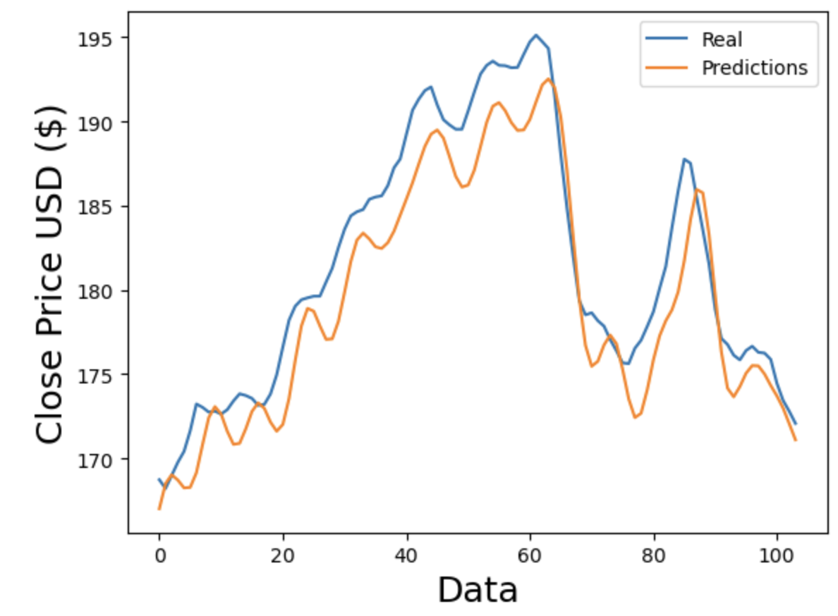
Figure 1. Comparing predictions and real value of Apple for LSTM (Photo/Picture credit: Original).

3. Results and discussion

After using the three datasets to train the LSTM and ARIMA models, predictions are compared to actual values in Fig. 1, Fig. 2, Fig. 3, Fig. 4, Fig. 5 and Fig. 6. For the same number of data points, Fig. 4, Fig. 5 and Fig. 6 show better adherence between predicted and real values visually, while Fig. 1, Fig. 2 and Fig. 3 show greater discrepancies between predicted and real values. Consequently, according to figures, ARIMA does a better job forecasting the stock prices of Apple, Microsoft, and Amazon. Since the RMSE and R² are indices to measure the performance of models statistically, Tables 2-4 compare the resulting RMSE and R² from the three stocks.

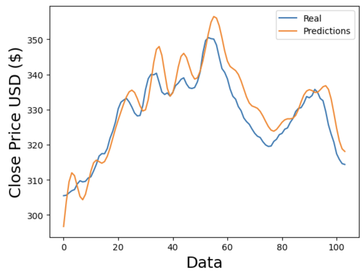
Figure 2. Comparing predictions and real value of Microsoft for LSTM (Photo/Picture credit: Original).

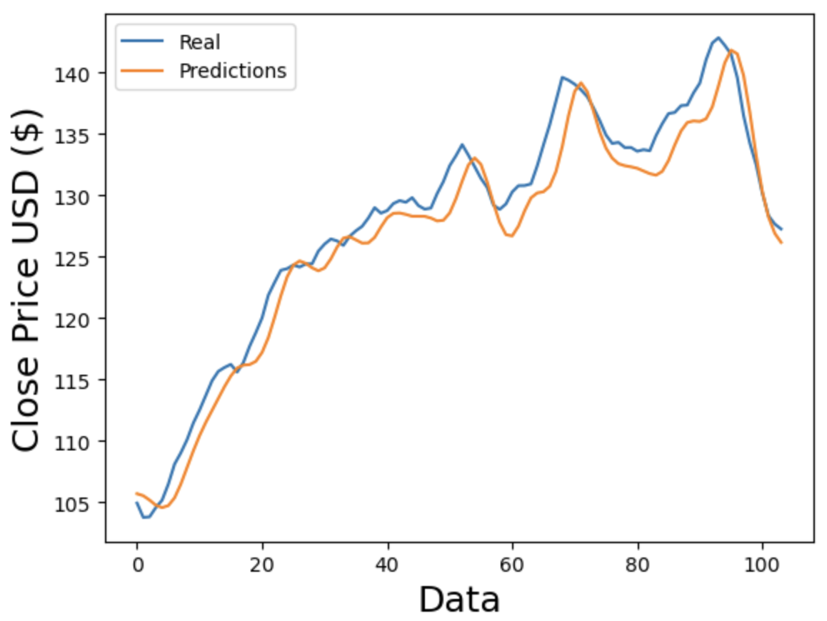
Figure 3. Comparing predictions and real value of Amazon for LSTM (Photo/Picture credit: Original).

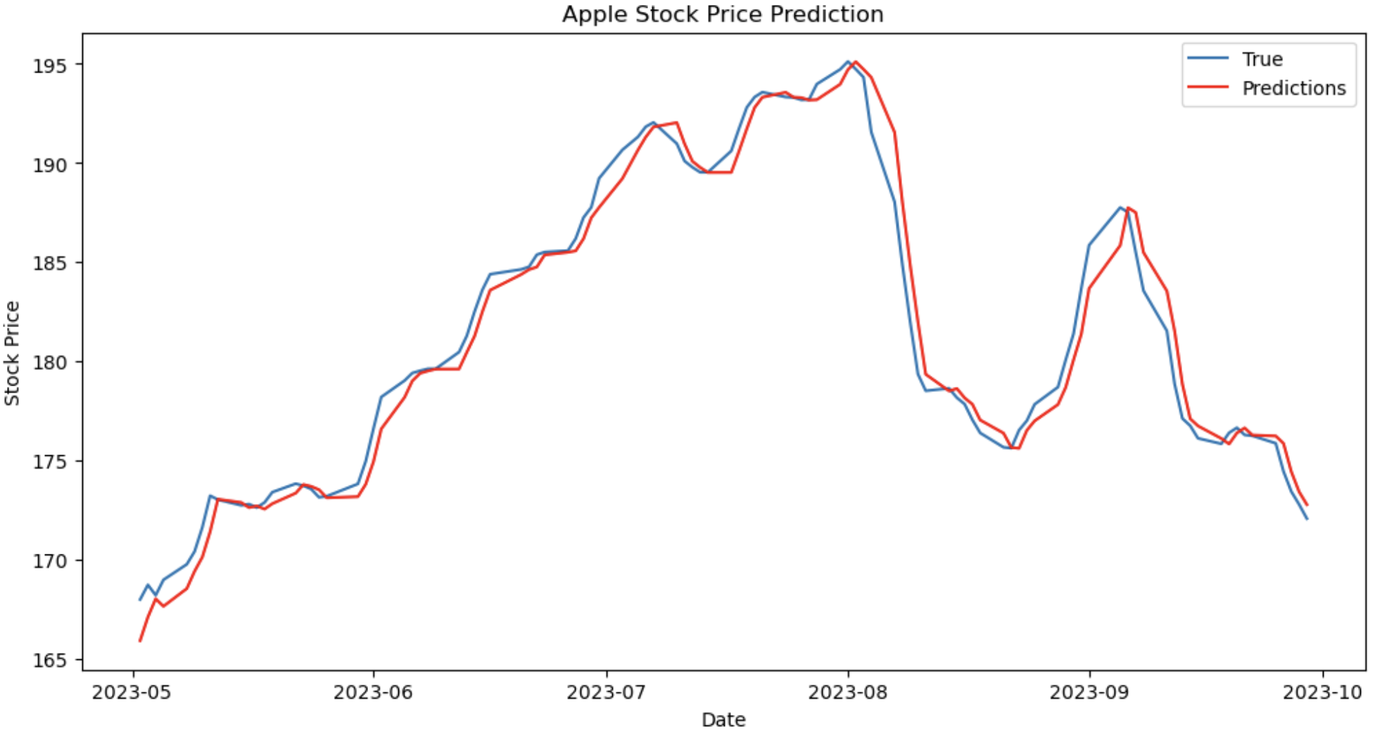
Figure 4. Comparing predictions and real value of Apple for ARIMA (Photo/Picture credit: Original).

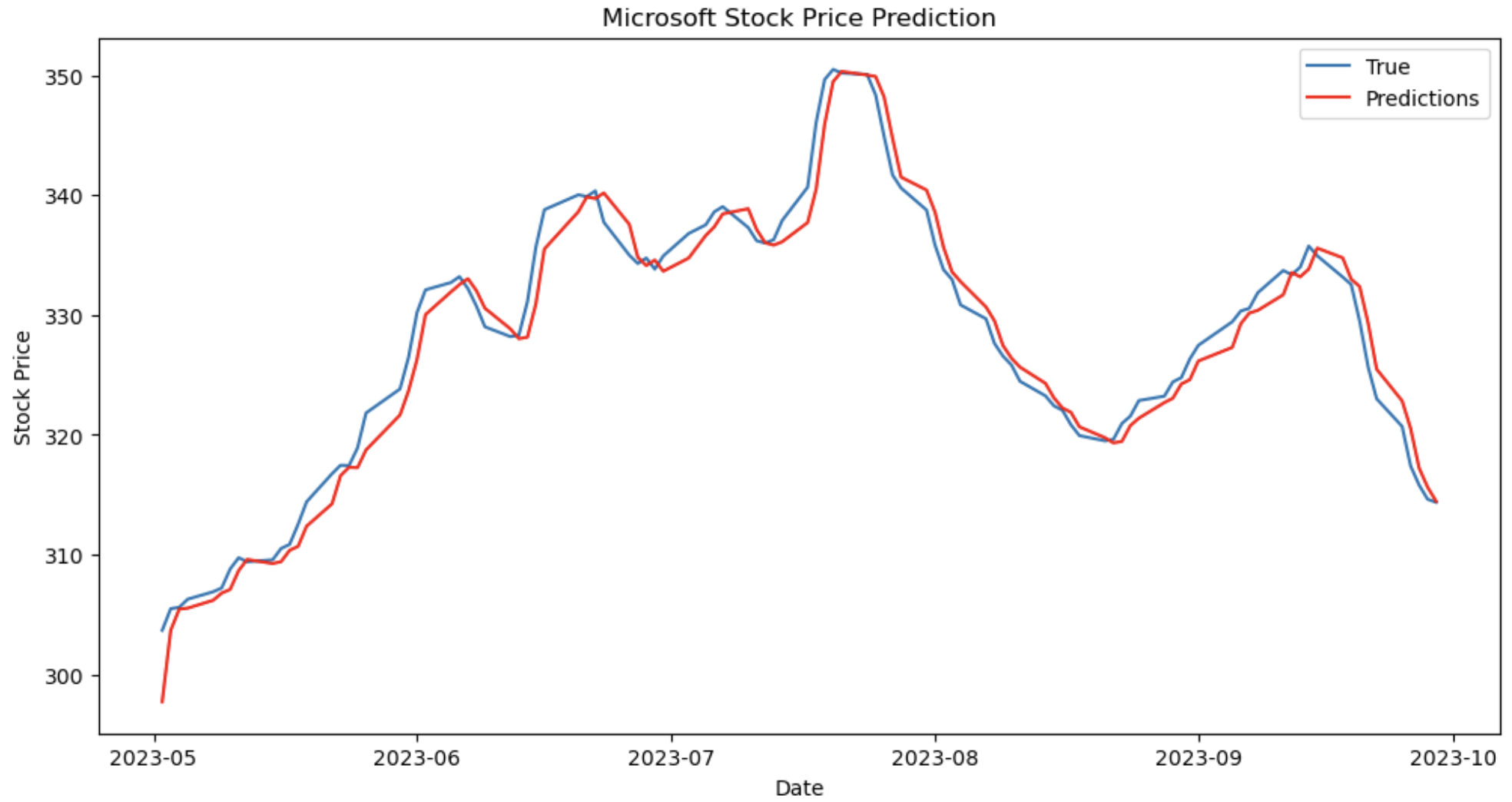
Figure 5. Comparing predictions and real value of Microsoft of ARIMA (Photo/Picture credit: Original).

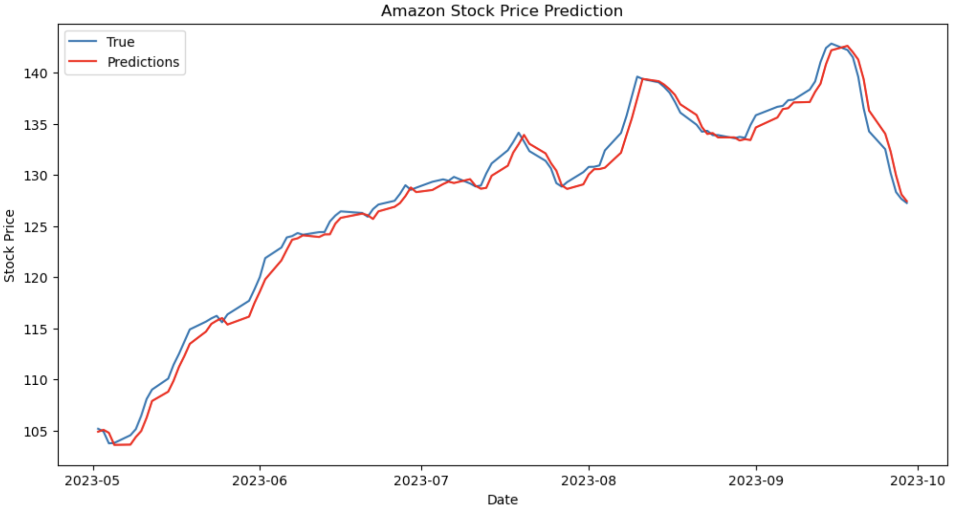
Figure 6. Comparing predictions and real value of Amazon for ARIMA (Photo/Picture credit: Original).

Table 2. Comparison of LSTM and ARIMA’s evaluation indices on Apple.

Table 3. Comparison of LSTM and ARIMA’s evaluation indices on Microsoft.

Table 4. Comparison of LSTM and ARIMA’s evaluation indices on Amazon.

The comparison results are given in Table 2, Table 3 and Table 4. Statistical evidence demonstrates the straightforward outperformance of ARIMA on all three stocks. For Apple’s stock, \( {R^{2}} \) obtained by LSTM indicates that 86.35% of the real data could be explained by the model. Considering that 0.85 is a common threshold to validate models, LSTM achieved efficiency in predicting Apple’s stock. ARIMA, on the other hand, obtained a \( {R^{2}} \) of 0.9769, meaning that 97.69% of the real data could be explained by its model. ARIMA’s RMSE is also significantly lower than LSTM’s, as a lower RMSE indicates smaller discrepancies between real data and predictions. ARIMA’s advantage is more obvious in predicting Microsoft’s stock. ARIMA has an \( {R^{2}} \) of 0.9715 and is considerably higher than LSTM’s \( {R^{2}} \) of 0.7806. Moreover, LSTM’s \( {R^{2}} \) has not passed the 0.85 threshold this time. ARIMA’s RMSE is also smaller than LSTM’s by a large extent, as ARIMA’s RMSE is 5.0984 and LSTM’s RMSE is 1.8729. Lastly, Both models’ performances are similar in Amazon’s stock. LSTM has an \( {R^{2}} \) of 0.9471 and ARIMA has an \( {R^{2}} \) of 0.9882. ARIMA achieved slightly better. From RMSE’s perspective, ARIMA outperforms LSTM again by having an RMSE of 1.0723, while LSTM has an RMSE of 2.2270. According to the results, the performance of ARIMA is outstanding among all three stocks and inherently indicates its consistency. However, this does not mean that the ARIMA used is flawless. Further investigations should be spent on preventing overfitting and detecting seasonality within the data. Moreover, there are various ways to improve LSTM, like different approaches to eliminate noise and including more features to train the model. This research does not indicate that ARIMA is generally a better model in stock price forecasting, but that the ARIMA used in the experiment is better than LSTM under designed conditions. Therefore, in predicting the stock prices of Apple, Microsoft, and Amazon, ARIMA outperforms LSTM.

4. Limitations and prospects

The analysis, while comprehensive, is not devoid of its limitations. First, the very nature of stock prices, being affected by an array of macroeconomic and company-specific factors, renders them highly non-linear and complex. The experiment only considered historical stock prices and their 5-day moving average, overlooking other potential influencers like trading volumes, macroeconomic indicators, or company-specific news. Secondly, while the ARIMA model showed superior performance compared to LSTM for the selected stocks, it doesn't guarantee consistent results across various other stocks or in different market conditions. ARIMA's underlying assumptions of linearity and stationarity could be a limitation in highly volatile markets or when sudden unexpected events (like geopolitical incidents or natural calamities) impact stock prices. Conversely, LSTM's capability to capture long-term dependencies might outperform ARIMA in more extended datasets. Third, sentiment analysis, as alluded to previously, is becoming an essential tool for stock prediction. The present study, however, did not integrate sentiment or other external data types into the models, which could have potentially improved forecasting accuracies.

Looking ahead, future endeavours should focus on hybrid models combining the strength of traditional time series forecasting techniques, like ARIMA, with the power of deep learning methods, such as LSTM. Incorporating more data types, especially sentiment data from sources like news articles, social media, or financial reports, can provide more holistic models. Exploring other machine learning algorithms, like reinforcement learning or attention mechanisms, may offer new insights. The burgeoning field of quantum computing also promises breakthroughs in time series analysis, given its potential for parallel computations. Furthermore, the continuous evolution of markets and trading strategies, coupled with technological advancements, mandates consistent re-evaluation and refinement of predictive models. In a landscape marked by frequent algorithmic trades and high-frequency trading systems, the durability of a model's predictive power is under constant scrutiny. Future research should also focus on real-time analysis and the potential of adaptive models that can adjust to new data quickly, ensuring relevancy in the ever-shifting terrain of stock markets. To conclude, while the presented models offer promising results in forecasting stock prices of the selected stocks, they underscore the intrinsic complexity and unpredictability of stock markets. Their future evolution will inevitably be interwoven with advancements in technology, offering both challenges and opportunities for market participants and researchers alike.

5. Conclusion

Predicting stock prices remains a perennial challenge in the financial realm. In this research, the forecasting accuracy of LSTM and ARIMA models was rigorously compared, focusing on the stocks of Apple, Microsoft, and Amazon. Findings revealed ARIMA's superior performance, as determined by RMSE and R² metrics, over LSTM. However, the study's limitation lies in the omission of external influencing factors and potential room for LSTM model optimization. Future endeavours might consider hybrid models or integrating broader datasets to enhance prediction precision. The significance of this study underscores the importance of selecting appropriate forecasting tools and facilitating more informed decision-making in the volatile domain of stock investments.

References

[1]. Lo, A. W. (n.d.). The Adaptive Markets Hypothesis: Market Efficiency from an Evolutionary Perspective.
[2]. Atsalakis, G., & K, V. (2013). Surveying stock market forecasting techniques - Part I: Conventional methods. (pp. 49–104).
[3]. Obthong, M., Tantisantiwong, N., Jeamwatthanachai, W., & Wills, G. (2020). A Survey on Machine Learning for Stock Price Prediction: Algorithms and Techniques: Proceedings of the 2nd International Conference on Finance, Economics, Management and IT Business, 63–71. https://doi.org/10.5220/0009340700630071
[4]. Beaudry, P., & Portier, F. (2004). Stock Prices, News and Economic Fluctuations (w10548; p. w10548). National Bureau of Economic Research. https://doi.org/10.3386/w10548
[5]. Degutis, A., & Novickytė, L. (2014). THE EFFICIENT MARKET HYPOTHESIS: A CRITICAL REVIEW OF LITERATURE AND METHODOLOGY. Ekonomika, 93(2), 7–23. https://doi.org/10.15388/Ekon.2014.2.3549
[6]. Khan, S., & Alghulaiakh, H. (2020). ARIMA Model for Accurate Time Series Stocks Forecasting. International Journal of Advanced Computer Science and Applications, 11(7). https://doi.org/10.14569/IJACSA.2020.0110765
[7]. Yan, X., Weihan, W., & Chang, M. (2021). Research on financial assets transaction prediction model based on LSTM neural network. Neural Computing and Applications, 33(1), 257–270. https://doi.org/10.1007/s00521-020-04992-7
[8]. Wu, J. M.-T., Li, Z., Herencsar, N., Vo, B., & Lin, J. C.-W. (2023). A graph-based CNN-LSTM stock price prediction algorithm with leading indicators. Multimedia Systems, 29(3), 1751–1770. https://doi.org/10.1007/s00530-021-00758-w
[9]. Lu, W., Li, J., Li, Y., Sun, A., & Wang, J. (2020). A CNN-LSTM-Based Model to Forecast Stock Prices. Complexity, 2020, 1–10. https://doi.org/10.1155/2020/6622927
[10]. Abraham, R., Samad, M. E., Bakhach, A. M., El-Chaarani, H., Sardouk, A., Nemar, S. E., & Jaber, D. (2022). Forecasting a Stock Trend Using Genetic Algorithm and Random Forest. Journal of Risk and Financial Management, 15(5), Article 5. https://doi.org/10.3390/jrfm15050188
[11]. Sonkiya, P., Bajpai, V., & Bansal, A. (2021). Stock price prediction using BERT and GAN (arXiv:2107.09055). arXiv. http://arxiv.org/abs/2107.09055
[12]. Hochreiter, S., & Schmidhuber, J. (1997). Long Short-Term Memory. Neural Computation, 9(8), 1735-1780.
Cite this article
Xia,X. (2024). Apple, Microsoft, and Amazon stock price prediction based on ARIMA and LSTM. Applied and Computational Engineering,53,181-189.
Data availability
The datasets used and/or analyzed during the current study will be available from the authors upon reasonable request.
Disclaimer/Publisher's Note
The statements, opinions and data contained in all publications are solely those of the individual author(s) and contributor(s) and not of EWA Publishing and/or the editor(s). EWA Publishing and/or the editor(s) disclaim responsibility for any injury to people or property resulting from any ideas, methods, instructions or products referred to in the content.
About volume
Volume title: Proceedings of the 4th International Conference on Signal Processing and Machine Learning
© 2024 by the author(s). Licensee EWA Publishing, Oxford, UK. This article is an open access article distributed under the terms and
conditions of the Creative Commons Attribution (CC BY) license. Authors who
publish this series agree to the following terms:
1. Authors retain copyright and grant the series right of first publication with the work simultaneously licensed under a Creative Commons
Attribution License that allows others to share the work with an acknowledgment of the work's authorship and initial publication in this
series.
2. Authors are able to enter into separate, additional contractual arrangements for the non-exclusive distribution of the series's published
version of the work (e.g., post it to an institutional repository or publish it in a book), with an acknowledgment of its initial
publication in this series.
3. Authors are permitted and encouraged to post their work online (e.g., in institutional repositories or on their website) prior to and
during the submission process, as it can lead to productive exchanges, as well as earlier and greater citation of published work (See
Open access policy for details).