1. Introduction

In recent years, thanks to the rapid development and increasing use of technologies such as multi-electrode and optical recording, researchers can record large-scale neural data with high resolution. Numerous scholarly investigations within the field of neuroscience have undergone a substantial shift in focus, transitioning from the study of individual neurons to the analysis of neural populations. This transition is driven by the acknowledgment that neural populations possess the ability to generate and convey a more extensive amount of information. Dimensionality reduction is always used to analyze neural population activity. This method can produce low-dimensional representations of high-dimensional data to preserve and highlight the neural mechanisms and statistical power underlying various phenomena [1].

Traditional methods, for example, PCA, are static dimensionality reduction methods which does not take into account time labels, and neural data are mostly time series. With the help of GPFA, researchers can leverage the time label information to get more powerful dimensionality reduction for time series data [2]. Nowadays, there are many existing studies about GPFA, which inspire a lot of different GPFA models based on different kinds of specific problems. One of the most famous applications is using GPFA to disentangle the bidirectional signal flow between two brain areas [3]. However, dimensionality reduction problems are countless. Even within the angle of neural data problems, there are still plenty of unknown latent dynamics. And it is unrealistic to set up unique GPFA models for each of them. Thus, setting up a commonly used GPFA model is necessary. Moreover, besides the large number of studies of the GPFA model, researchers do not have a useful way to determine the hyperparameter, or in other words, the dimension of the latent, which is a big problem in using the GPFA model.

This paper aims to propose a new and common framework for GPFA to cover the whole process of neural data analysis. Since the linear combination of Gaussian distribution can simulate all kinds of probability distribution [4], this framework will use the standard GPFA model to fit the unknown neural dynamics. With the help of the method of expectation-maximization, the speed of fitting the model can be dramatically increased. Then, by using a novel approach of spanning all the possible latent dimension values by cross-validation, the most suitable hyperparameter will be found. To guarantee the utility of the framework, in this paper, the framework will be used on the synthetic data generated by the generative model at first. After checking the results of reproducing the spike rate sequence and the most suitable model on the synthetic data, the model will be applied to a real neural dataset recording from the V1 area of anesthetized macaque monkeys.

2. Method

2.1. Data

The neural data used in this paper is a multi-electrode recording data recorded from anesthetized macaque monkeys. In the experiment, natural images and gratings were flashed on the screen, and meanwhile, the multi-electrode recorded the activity in monkey’s brains. The whole dataset can be split into two parts, the first part was the brain activity when monkeys were shown the images, and the other part was the one after being shown the images. This paper uses the second part of the dataset because it can ensure a coherent process in a monkey’s brain. The data is a 3-D array in the form of #trials#neurons#miliseconds, including 20 trials, 102 neurons, and 211 millisecond time points. The value of each data point is binary, either 0 or 1, which suggests whether there is a neural spike in the time point or not. The data was posted to CRCNS.org on November 23, 2015, and labeled as primary visual cortex number 8 [5].

2.2. Model

To sum up, the whole framework can be divided into two parts: fitting the GPFA model and choosing the hyperparameter. Each part will be described below. The whole work in this paper can also be split into two steps: validating the synthetic data and applying it to the real neural data.

In neuroscience, when the membrane potential of a neuron reaches a threshold, it will generate a sudden increase which is called a spike. There are two ways to record the information of neural activity: the first one is the spike train, which contains the spiking time of each neuron; the second one is the spike rate, which is defined as the number of spikes within a short time. The width of a time bin can have different choices and will lead to different results. Researchers often use spike binning square root transform to convert a spike train into the form of a spike rate. The framework is based on the standard GPFA model [6].

\( Y=CX+d+N(0, R \) \( ) \) (1)

Where Y is a matrix in the shape of M×T, where M stands for the number of neurons and T represents the total amount of time points. Each point in the Y matrix is the spike count of a neuron at a time point. The basic idea of GPFA is to find the projection of the matrix Y in a low-dimensional subspace. And C is the transform matrix in the shape of M×P. X is the latent structure of the GPFA model in the shape of P×T, where P is the dimension of the latent. To make it close to reality, this model also adds the bias d and the Gaussian noise N ~ (0, R). The goal is to fit the model to an unknown neural structure. The method expectation-maximization is usually the first choice to do the fitting work which has proved to be an accurate and fast approach compared with some traditional methods such as stochastic gradient descent.

The spike counts are not necessarily a positive value. To convert the spike count, which is the value of each point of the matrix Y, into a non-negative spike rate, a simple math trick is needed:

\( spike rate= {(70Hz)^{{y_{i,j}}/((Y))}} \) (2)

Where \( {y_{i,j}} \) is a value point of the matrix Y.

The next part of the framework is to tune the hyperparameter, or in other words, choose the best latent dimension value. Some existing methods such as likelihood ratio tests may be very complicated and depend on some specific conditions, and using Cross-Validation can successfully avoid such problems and overfitting [7]. The idea here is to calculate the validation for each possible value of the latent dimension and choose the one with the highest value. Since the Bayesian Marginal log-likelihood can be equivalent to the Cross-Validation score using the log posterior predictive probability as the scoring rule [8], it is reasonable to average the marginal log-likelihoods for each fold of the Cross-Validation as the validation or score.

The first step in this paper is to validate the model on the synthetic data. The synthetic data is generated by the generative model which shows the spike rate of each neuron at each time point. The generative model is a modified GPFA model. The reason why modifying the model is to make it more real. According to the definition of spike rate, it should be a non-negative value. The latent structure X of the model is a traditional Gaussian process. Add the exponential function to each element of the projection matrix after projecting to the high dimensional space by the transform matrix W [9]:

\( Y=exp⁡(WX \) \( ) \) (3)

Therefore, each element of the matrix Y becomes equal to or greater than zero. Because the count of the neural spikes is integer, it is obviously that an inhomogeneous Poisson Process can be approximated to the distribution of spike train. The following work is to fit the standard GPFA model to the spike train. After getting the parameters C, d, and R, it is time to reproduce the sequence of spike rate and spike train. Another thing is to check the suitable hyperparameter. All of the results will be compared with the initial setting of the generative model, which is the validation of the framework.

The next step is to apply this framework to the real neural data of the anesthetized macaque monkeys. The process is similar to the work on the synthetic data: fitting the standard model with expectation maximization and getting the parameters, checking the appropriate latent dimension with cross-validation, and reproducing the spike rate and the spike train. The only difference is that because the form of the neural data is binary, which means each value point is either one (spike) or zero (silence), the neural data should be preprocessed and converted into the form of showing the exact time of spikes. After this transformation, it can be compatible with the algorithm.

2.3. Evaluation

Three things need to be evaluated: the accuracy of the reproduced spike rate, the reproduced latent, and the reproduced latent dimension. If the difference between the real latent dimension and the reproduced one is no more than two, it will be a reasonable result. And for the first and second one, currently, there is no appropriate method to measure the accuracy. But after plotting the reproduced one and the real one, it is possible to compare the number and the position of the peak to show how much the reproduced one fits the real one. Moreover, there are also two ways to reproduce the spike rate: one is to directly use the parameters to reproduce the standard GPFA model; and the other is to follow the structure of the generative model. Seeing that the latent in the two models have the same definition, it is necessary to check both of them.

3. Result

3.1. Synthetic data

The synthetic data is generated by the model mentioned in the last section. To show the latent dynamics more vividly, the dimension of the latent was chosen as two dimensions. That is because two dimensions can directly be posted on a plane. This study constructs a projection from two latent to fifty neurons. The parameters here are the transform matrix W and kernel parameter l, where the kernel is radial basis function kernel

\( exp⁡(-{({t_{1}}-{t_{2}})^{2}}/(2{l^{2}} \) \( ) \) (4)

The results of the generative data are shown in Figure 1.

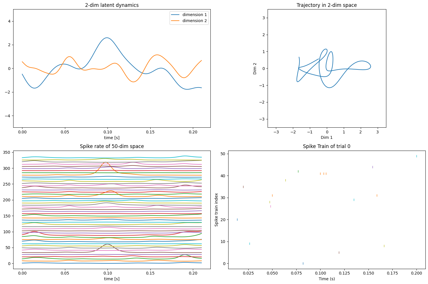
Figure 1. Visualization of the generated data. Upper left: The low-dimensional latent structure; Upper right: the trajectory of latent dimension in 2-d picture; Lower left: the spike rate of each neuron in the generated data; Lower right: the spike train of the generated data.

The first task is to reproduce the spike rate by using the standard GPFA model. And the first step is to use EM (expectation-maximization) method to fit the data by the standard model. After getting the parameters, using equation (1), (2) to reproduce the spike rate, and the result is shown in Figure 2. The picture on the left-hand side of Figure 2 is the real spike rate, and the one on the right-hand side is the reproduced spike rate. It is obvious that the real one is smoother and the difference between these two is non-trivial.

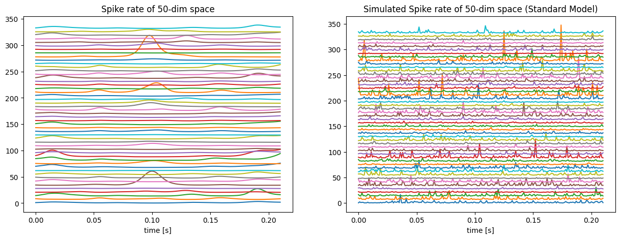
Figure 2. Comparison of the synthetic spike rate (left) and the spike rate reproduced from the standard model (right).

However, after applying these two to an inhomogeneous Poisson Process and generating the spike train which is shown in Figure 3, it seems that the difference between the real one and the reproduced one is not as large as the spike rate. Figure 3 suggests that there are a total of 18 spikes in the original data and 16 spikes in the generated spike train, and the degree of dispersion of the two spike train results are very similar. Since the generative model and the fitting model are two completely different models, it is rational to believe that there are two different ways leading to the same result by the inhomogeneous Poisson Process, and the final result here is the spike train. Always remember that the final target is to reproduce the spike train, not the spike rate.

Figure 3. Comparison of the synthetic spike train (left) and the spike train reproduced from the standard model (right).

Let’s move on to the next task: reproducing with the generative model. The latent sequence X remains but is applied to the generative model by using the equation (3). Figure 4 shows an even much larger difference than Figure 2. It may be because using another model to fit the result will bring much more error. Regarding the structures of the two models, it is easy to find out that the standard model dramatically amplifies the value of the latent by the exponential of 70 Hz, which is much larger than the generative model with the exponential of Euler number. So, when reproducing the spike rate with the generative model, its fluctuation will be much smaller than before.

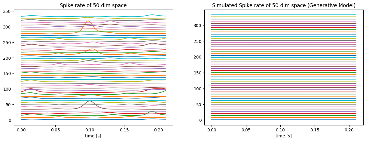
Figure 4. Comparison of the synthetic spike rate (left) and the spike rate reproduced from the generative model (right).

Nevertheless, checking the reproduced spike train is necessary to validate the idea that reproducing from the generative model is not rational. Figure 5 shows that reproducing from the generative model also cannot generate a similar spike train with the original data, neither the frequency of the spikes nor the neuron generating a spike. To sum up, although getting a much different spike rate, the framework of the standard model can successfully reproduce a similar spike train with the original data. On the other hand, directly using the generative model will not receive a good result no matter in spike rate or spike train.

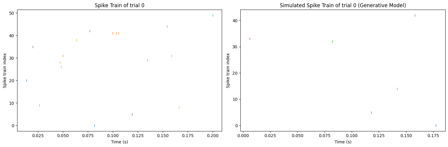
Figure 5. Comparison of the synthetic spike train (left) and the spike train reproduced from the generative model (right).

The final task is to use the cross-validation to find the suitable hyperparameter. From Figure 6, it is obvious that the result is three, which satisfies the demand of difference no more than two. It shows that the cross-validation part of the framework works. So far, the framework shows a robust effect on the synthetic data, and it is time to apply it to the real neural data.

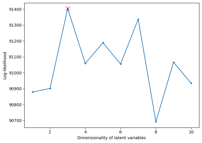
Figure 6. Log-likelihood of each possible value of the latent dimension of the synthetic data.

3.2. Real Neural Data

After a simple preprocessing, the real neural data from the anesthetized macaque monkeys is shown in the form in Figure 7. The first step in this section is to find the suitable latent dimension. Just repeat the steps in section 3.1, and the result is shown below in Figure 8.

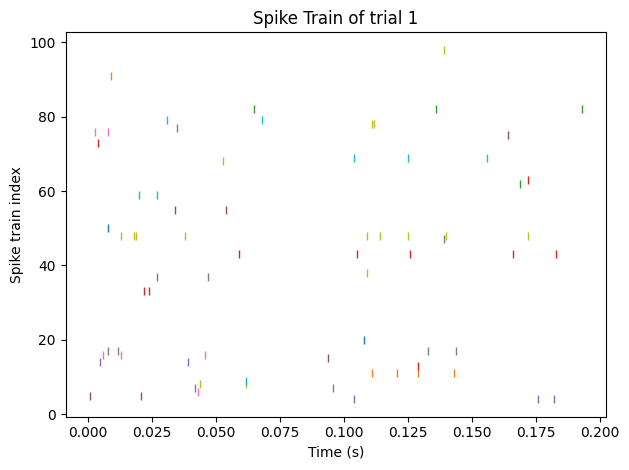
Figure 7. Visualization of the spike train after preprocessing.

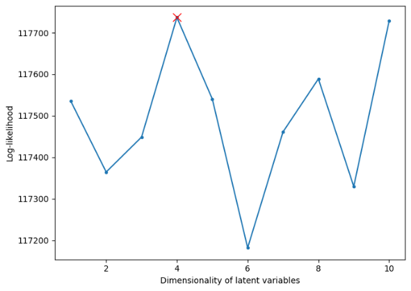
Figure 8. Log-likelihood of each possible value of the latent dimension of the real neural data.

The dimension of the latent is three. Thus, in the following steps, the latent dimension parameter should be set as three. According to the conclusion in section 3.1, it is nonsense to think about the underlying structure of the neural activity since the standard GPFA model has already fitted the spike train. Then, reproduce the spike train with the help of parameters inferred from the standard GPFA model.

Figure 9 shows that there are still some differences between the final result and the original data. The original data shows a little bit more spikes and more spiking neurons than the reproduced data, which means that the framework still needs to be optimized. In the next section, some more details of the framework will be analyzed and discussed, aiming to find some new directions for future studies.

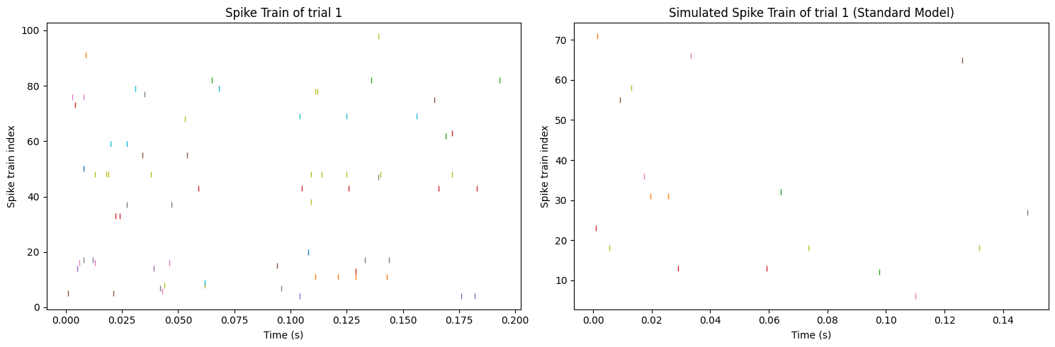
Figure 9. Comparison of the real neural spike train (left) and the spike train reproduced from the standard model (right).

4. Discussion

The framework proposed in this paper has a good performance on the synthetic data, however, it still cannot meet the expectations of the real neural data. It shows that there are still some limitations in this framework, and it is worthwhile to discuss the reason for them.

One of the biggest problems of this framework is that there is no ready-made method to determine or measure the accuracy of the framework. Most of the comments on the result are based on the intuition of the naked eye. It is possible to compare two methods of reproducing with the model data and figure out which one is better, however, when it comes to a single result and model data, intuition is not correct. Thus, setting up a rule for analyzing the similarity between two spike trains is necessary.

The framework also has some details that need to be studied. For example, the kernel used to create the Gaussian process of the latent structure X. This paper uses the radial basis function kernel because it is the most commonly used one [10]. But it is still uncertain whether it is the best choice or not. Moreover, when projecting the latent dynamics X to the high-dimensional space, a math trick is always needed to get a positive value of the spike rate matrix Y, and there is no certain way to do such a math trick. Even in this paper two different approaches. These two problems are worth studying in the future since they are correlated heavily with the framework.

Finally, a possible reason that this framework performs better on the synthetic data is that the generative model is still a slightly modified GPFA model, which may share some common features with the standard GPFA model. In this case, the framework needs to be more precise to adapt to some models that are not as Gaussian as the generative model used in this paper.

5. Conclusion

This paper aims to propose a generic framework that can adapt to most kinds of neural data and neural activity, finding the latent structure and reproducing the spike train. The framework is based on the standard Gaussian-Process Factor Analysis model. With the help of an expectation-maximized algorithm, this model can be quickly embedded into the spike train and get the parameters. The innovative part is the method of choosing the appropriate latent dimension by spanning all the possible values using cross-validation. This framework performs well on the synthetic data. It roughly reproduces the original spike train in both frequency and spiking neurons. It also successfully finds the closed value of the latent dimension by calculating the average log-likelihood. However, it still shows some limitations on the real neural data. The final result shows clear differences with the original spike train. Fortunately, this work does not work into a dead end. There are still some parts that can be improved, for example, the kernel function of the covariance matrix, the method of converting the spike count into a non-negative spike rate, and most importantly, a standard that can measure the accuracy of the model and the spike train. These shortages mean that this framework has the potential to become better. On the other hand, a wilderness demand for such kinds of models will push the development of the GPFA model. The applications of the GPFA model are wide in neuroscience. Therefore, this kind of model will continuously draw strong attention from neuroscientists and there will always be someone trying to improve the performance of it. Hope that with the development of the relevant technology, a more useful GPFA model can be developed soon.

Acknowledgments

The data were collected in the Laboratory of Adam Kohn at the Albert Einstein College of Medicine and downloaded from the CRCNS web site.

References

[1]. John P C and Yu B M 2014 Dimensionality reduction for large-scale neural recordings Nature neuroscience 17(11) pp 1500–1509
[2]. Yu B M, John P C, Santhanam G, Ryu S I, Shenoy K V, and Sahani M 2009 Gaussian-process factor analysis for low-dimensional single-trial analysis of neural population activity Adv neur inf proc sys pp 1881–88
[3]. Gokcen, E., Jasper, A.I., Semedo, J.D. et al. 2022 Disentangling the flow of signals between populations of neurons Nat Comput Sci 2 pp 512–525
[4]. Bialek, W. 2020 What do we mean by the dimensionality of behavior. arXiv: Neurons and Cognition
[5]. Ruben Coen-Cagli, Adam Kohn, Odelia Schwartz 2015 Flexible Gating of Contextual Influences in Natural Vision Nature neuroscience 18 pp 1648-55
[6]. Bruinsma, W.P., Perim, E., Tebbutt, W., Hosking, J.S., Solin, A., & Turner, R.E. 2019 Scalable Exact Inference in Multi-Output Gaussian Processes. ArXiv, abs.1911.06287
[7]. Richie, R., & Verheyen, S. 2020 Using cross-validation to determine dimensionality in multidimensional scaling Computer Science
[8]. E Fong, CC Holmes 2020 On the marginal likelihood and cross-validation. Biometrika, 107(2) pp 489–496
[9]. SL Keeley, DM Zoltowski, Y Yu, JL Yates, SL Smith, & JW Pillow 2020 Efficient Non-conjugate Gaussian Process Factor Models for Spike Count Data using Polynomial Approximations. In H. Daume, & A. Singh (Eds.), 37th International Conference on Machine Learning, ICML pp 5133-5142
[10]. Pandarinath, C., O’Shea, D.J., Collins, J. et al. 2018 Inferring single-trial neural population dynamics using sequential auto-encoders. Nat Methods 15 pp 805–815
Cite this article
Xu,T. (2024). Inferring the latent low-dimensional structure of unknown neural dynamics with standard Gaussian-Process Factor Analysis framework. Applied and Computational Engineering,55,14-22.
Data availability
The datasets used and/or analyzed during the current study will be available from the authors upon reasonable request.
Disclaimer/Publisher's Note
The statements, opinions and data contained in all publications are solely those of the individual author(s) and contributor(s) and not of EWA Publishing and/or the editor(s). EWA Publishing and/or the editor(s) disclaim responsibility for any injury to people or property resulting from any ideas, methods, instructions or products referred to in the content.
About volume
Volume title: Proceedings of the 4th International Conference on Signal Processing and Machine Learning
© 2024 by the author(s). Licensee EWA Publishing, Oxford, UK. This article is an open access article distributed under the terms and
conditions of the Creative Commons Attribution (CC BY) license. Authors who
publish this series agree to the following terms:
1. Authors retain copyright and grant the series right of first publication with the work simultaneously licensed under a Creative Commons
Attribution License that allows others to share the work with an acknowledgment of the work's authorship and initial publication in this
series.
2. Authors are able to enter into separate, additional contractual arrangements for the non-exclusive distribution of the series's published
version of the work (e.g., post it to an institutional repository or publish it in a book), with an acknowledgment of its initial
publication in this series.
3. Authors are permitted and encouraged to post their work online (e.g., in institutional repositories or on their website) prior to and
during the submission process, as it can lead to productive exchanges, as well as earlier and greater citation of published work (See
Open access policy for details).