


1. Introduction
With the advancement of technology, the multi-robot technology has been increasingly valued by people. The area coverage task requires the robot to avoid obstacles in the area and continuously explore the environment, sensing and recording the surrounding environment through sensors until the robot traverses the entire area and collects environmental information for the entire area. Coverage tasks typically require exploring unknown environments, facing unknown obstacles, and spending a lot of time. Multi-robot possess collaborative capabilities, high flexibility and work efficiency. So multi-robot is widely used in coverage tasks, such as implement sensor coverage in an environment that rejects communication [1], perform fast environment mapping [2], [3], search and rescue [4] and so on. When the scale of the environment and robot teams are not large, management and control of the robot population can be achieved easily. But as the scale and complexity of the environment become large, the implementation difficulty of robot coverage algorithms greatly increase. This is because in real life, many data are generated from non-Euclidean spaces, and most of the data represents graphs with complex relationships and interdependent relationships between objects. The performance of traditional deep learning methods in processing complex graph data is not optimistic because the graph is irregular and complex. This inspires us to solve the problem using another method that is suitable for processing graph data. That is graph neural networks (GNN).
Recently, Graph Neural Network (GNN) is widely used in multi-robot problem. Such as path planning [5],[6], search [7] and rescue, etc. These works inspire us to use Graph Neural Networks (GNN) to solve coverage tasks. When multi-robot needs to handle coverage problems, according to [8], we understand that firstly, robots need to access a set of locations in the environment. When we use graph neural networks (GNN) to solve the coverage problems, we first encode the multi-robot coverage task, extract graph data from non-Euclidean space, then convert the task into a graph. In global agents, each robot is regarded as a node in the graph. The allowed movement is the graph edge. With this method, we can abstract the entire map and obstacle model. And we can show all the elements of the problem in a single spatial map. The elements only have local links [9].
When we need to solve muti-robot path planning problems, we can imitate expert solutions. The existing research can already support medium team size coverage tasks. We can collect task data and expert solutions. And then use these data to train GNN controllers to learn and imitate experts. After that, it can be extended to larger teams and maps. In [9], the generalization of the scene simulating a quadcopter aircraft is demonstrated. This environment has thousands of waypoints. The quadcopter aircraft must traverse them. Furthermore, this approach is applied to the exploration task. But robots will show team waypoint maps during task execution. This scene prove that the graph neural network controller can perform heuristic learning by learning and imitating experts. And the trained graph neural network controller performs well.
In this article, we also designed a GNN architecture. This GNN architecture that abstracts using graph equivariance design. In this way we can accelerate learning progress. This way also can get zero shot generalization for large maps and teams can be achieved in this way [9]. And the graph neural network has more graph operation layers, which can enable the graph neural network controller to control long-distance information. The number of graph operation layers is directly related to the distance that information is transmitted from one node to another along the graph edge. To let the multiple robots explore as many areas of interest as possible within the limited time [10], this study will divide the map into multiple lattices and connect adjacent spatial nodes. Accelerate robot exploration efficiency by discretizing as many regions of interest as possible.
2. Method
2.1. Multi-Robot Coverage Problem
In this article, the robot set is defined as \( R \) , with all waypoints as \( W \) , unreachable waypoints as \( X \) , and \( X ⊆ W \) . Then, we define the environment map’s factors: \( {p^{j}} \) represents the position of the waypoint \( j \) . \( {N^{j}} \) represents all waypoints which is adjacent the waypoint \( j \) [9]. Then define \( x_{t}^{j}∈\lbrace 0,1\rbrace \) represents the interest of waypoint \( j \) at time \( t \) . If \( j∈ X \) , then \( x_{t}^{j} \) =1. \( T \) is the time of the task. The robot \( i \) position at time \( t \) is \( q_{t}^{i} \) [9]. If the robot is currently on waypoint \( j \) , then there is \( {1_{q_{t}^{i}={p^{j}}}} \) . We expressed the problem as [9]:
\( \begin{matrix}max \\ {\lbrace q_{t}^{i}\rbrace _{i∈R}} \\ \end{matrix}\sum _{t=0}^{T}\sum _{j∈W}\sum _{i∈R}x_{t}^{j}{1_{q_{t}^{i}={p^{j}}}}\ \ \ (1) \)
\( s. t. x_{t}^{j}=x_{0}^{j}\prod _{j∈W}\prod _{D0}^{t-1}(1-{1_{q_{t}^{i}={p^{j}}}}), ∀ j ∈ W ,t ≤ T\ \ \ (2) \)
\( {q_{t-1}^{i}=p^{j}},{q_{t}^{i}=p^{k}}⇒k ∈ {N^{j}} , ∀ i∈ R,∀ j, k ∈ W, t ≤ T\ \ \ (3) \)
The goal of this study is to design a controller with closed-loop. It will use heuristic learning to calculate the robot’s action based on the system state [9]. It can also perform generalization of dynamic graphs. This is beneficial for us to solve exploration problems, as robots can also discover new waypoints during the task. We attempt to learn another controller which also with closed-loop, π, which maximizes the expected waypoints on initial states and maps [9]:
\( \begin{matrix}Max \\ Π \\ \end{matrix} {E_{q_{0}^{i}{,p^{j}},x_{0}^{j},}}\sum _{t=0}^{T}\sum _{j∈W}\sum _{i∈R}x_{t}^{j}{1_{q_{t}^{i}={p^{j}}}}\ \ \ (4) \)
\( s. t. x_{t}^{j}=x_{0}^{j}\prod _{j∈W}\prod _{s=0}^{t-1}(1-{1_{q_{t}^{i}={p^{j}}}}), ∀ j ∈ W ,t ≤ T\ \ \ (5) \)
\( {q_{t-1}^{i}=p^{j}},{q_{t}^{i}=p^{k}}⇒k ∈ {N^{j}} , ∀ i ∈ R,∀ j, k ∈ W ,t ≤ T.\ \ \ (6) \)
\( {\lbrace q_{t}^{i}\rbrace _{i∈R}}=Π({\lbrace q_{t-1}^{i}\rbrace _{i∈R}}{\lbrace q_{t-1}^{i}\rbrace _{j∈W}}{\lbrace {p^{j}}\rbrace _{j∈W}})\ \ \ (7) \)
2.2. The coverage task
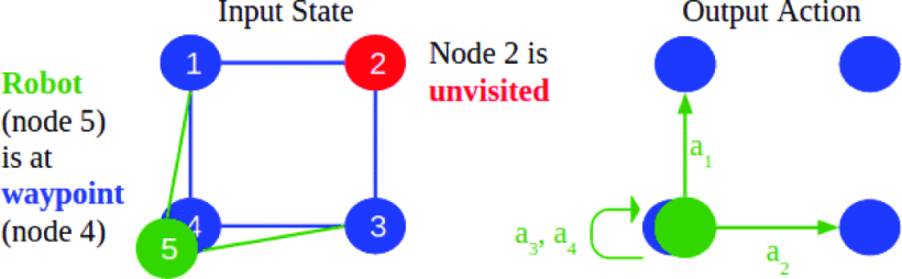
We abstract the agent and map and represent regard the robot as a node. The robot will move between nodes in a discrete form. The robot's action space is also discrete. Each robot will select one node around itself to move according to the learning algorithm. The topological structure of the graph will change as the robot moves. We use the lattice to abstract the global position of the robot. In order to reduce computational costs, we only maintain information between nodes and robots. In abstract graphics, there are two types of edges. They are (1), (2), (3) The edges between nodes are used to display the space covered and (4), (5), (6), (7) The edge between the robot and the node allows the robot to move to nearby nodes. We use the obstacles and the lattice induced on the map to defined the connectivity of waypoints. If \( {q_{i}}={p_{j}} \) ,then \( {N_{i}}={N_{j}} \) [9].
Each node type is represented by the index i of its feature vector \( { v_{i}} \) , 1 is the indicator function:
\( { v_{i}}=\lbrace {1_{i∈R}}{,1_{i∈W}}{,1_{i∈X}}\rbrace \ \ \ (8) \)
\( \) We define \( {e_{k}} \) is the feature vector of the index \( K \) ’s directed edge. \( {s_{k}} \) and \( {r_{k}} \) are the sender node and the receive node. \( {e_{k}} \) is distance \( {s_{k}} \) and \( {r_{k}} \) between node positions [9]. So the distance can be expressed:
\( {e_{k}}=‖{p_{{s_{k}}}}-{p_{{r_{k}}}}‖\ \ \ (9) \)
Among them, \( {e_{k}} \) is the feature vector of the index \( K \) ’s directed edge. \( {s_{k}} \) and \( {r_{k}} \) are the sender node and the receive node. \( {e_{k}} \) is distance \( {s_{k}} \) and \( {r_{k}} \) between node positions [9].
All edge elements is \( E= \lbrace {e_{k}}\rbrace \) , All vertex elements is \( V = \lbrace {v_{i}} \rbrace \) , and the graph representation of the system state is \( G = \lbrace E, V\rbrace \) . At time t, the task state is \( {G_{t}} \) [9]. The Figure.1,2 and 3 show that the training model was tested in Unity on a simulated robot team.
|
|
|
Figure 1. (a)Simulation of the city in Unity [9]. | Figure 2. (b) The graph represention of the task [9]. | Figure 3. (c)Ateam of 10 such quarotors were used [9]. |
|
Figure 4. The robot and the waypoint are the nodes and the edges indicating that the robot can move to different place [9]. |
2.3. The exploration task
We have represented the coverage graph, which has many waypoints. The process of robot exploration is the process of robots observing waypoints through sensors. In [9], when waypoints are observed by sensors in the range S, they will be added to the graph: if \( ‖p_{t}^{i}-q_{t}^{i}‖≤S \) , then \( {W_{t+1}}{=W_{t}}\bigcup \lbrace {p_{i}}\rbrace \) As time goes by, the degree of robot exploration will increase, and the number of waypoints in the waypoint concentration will increase.
In addition, we define nodes that may have unexplored adjacent nodes as boundary nodes. To distinguish whether a node is a boundary node, we add an indicator feature F to distinguish [9]:
\( { V_{i}}=[{1_{i∈R}}{,1_{i∈W}}{,1_{i∈X}},{1_{i∈F}}]\ \ \ (10) \)
2.4. Aggregation Graph Neural Networks
The GNN is one of the most widely used tools in the field of building system structures. Because the GNN can exploit the known structures of the relational system [11]. Graph convolutional networks are a type of GNNs. The graph convolution operation is defined by learnable coefficients, which multiply the power of the adjacency matrix by the graph signal [12], [13]. We will construct a multi robot system network architecture by merging nonlinear graph convolutional network operations [9]
Graphical network blocks are used to construct the basic structure of the system. Given a graphic signal, defined as \( G=\lbrace \lbrace {e_{k}}\rbrace ,\lbrace { v_{i}}\rbrace \rbrace \) , so \( G \prime = G=\lbrace \lbrace e_{k}^{ \prime }\rbrace ,\lbrace v_{i}^{ \prime }\rbrace \rbrace \) [9]:
\( E_{k}^{ \prime }={Φ^{e}}({e_{k}} {,v_{{r_{k}}}} ,{v_{{s_{k}}}}), v_{I}^{ \prime }={Φ^{v}}(\overline{e}_{I}^{ \prime } {,v_{I}} ,{v_{{s_{k}}}}), \overline{e}_{I}^{ \prime }={ρ^{e→v}}. \ \ \ (11) \)
\( GN (•) \) is the function \( G \) of the graphic signal. \( G \prime \) is \( {Φ^{e}} \) , \( {ρ^{e→v}} \) and \( {Φ^{v}} \) The graphic signal converted in this order. \( G \) and \( G \prime \) have the same connectivity.
The aggregation operation \( {ρ^{e→v}} \) adopts a set of transformed event edge elements \( E_{i}^{ \prime }{=\lbrace e_{k}^{ \prime }\rbrace _{{r_{k}}=i}} \) at node \( i \) and generates a fixed size latent vector \( \bar{e_{i}^{ \prime }} \) [9]. The function must be capable of processing various levels of graphics. Therefore, we normalize the output by aggregating the mean according to the number of input edges [9]:
\( {Ρ^{e→v}}(E_{I}^{ \prime })≔\frac{1}{|E_{I}^{ \prime }|}\sum _{e_{k}^{ \prime }∈E_{I}^{ \prime }}e_{k}^{ \prime }.\ \ \ (12) \)
In addition, we understand that mean aggregation operations can help improve the stability of GNNs with large receptive fields. We have designed two variants based on the aggregated GNN architecture of [14]. Linear Aggregated GNN architecture Linear and nonlinear Aggregated GNN architecture.
The linear aggregation GNN architecture can be represented by the following parameters:
\( Φ_{L}^{e}({e_{k}} {,v_{{r_{k}}}} ,{v_{{s_{k}}}})≔{v_{{s_{k}}}}\ \ \ (13) \)
\( Φ_{L}^{v}(\overline{e}_{I}^{ \prime }{,v_{i}})≔\overline{e}_{I}^{ \prime }\ \ \ (14) \)
Nonlinear aggregation GNN is represented by learnable nonlinear functions:
\( Φ_{N}^{e}({e_{k}} {,v_{{r_{k}}}} ,{v_{{s_{k}}}})≔N{N_{e}}([{e_{k}} {,v_{{r_{k}}}} ,{v_{{s_{k}}}}])\ \ \ (15) \)
\( Φ_{N}^{v}(\overline{e}_{I}^{ \prime } { ,v_{i}})≔N{N_{v}}([\overline{e}_{I}^{ \prime } { ,v_{i}}])\ \ \ (16) \)
Among them, there are 16 hidden units of 3-layer MLP. Note that, in contrast to the nonlinear GNN defined in (13), (14), a linear aggregate GNN in (9) may not use input edge characteristics, for example as defined in (15), (16) [9].
2.5. Policy Architecture
For the coverage problem, we have developed GNN variants with multiple stages. By connecting the outputs of each stage and finally processing them through linear output transformation [14]:
\( {G^{ \prime }}={f_{out}}([{f_{dec}}({f_{enc}}(G)),{f_{dec}}(GN({f_{enc}}(G))),{f_{dec}}(GN(GN({f_{enc}}(G)))),…])\ \ \ (17) \)
The number of GNN operations is a hyperparameter that determines the receptive field (K) of the architecture. K represents the distance that information can be transmitted along the edges of the graph. The \( {f_{enc}} \) , \( {f_{dec}} \) are 3layer MLPs with 16 hidden units. The \( {f_{out}} \) is a linear function. We sample the edges of each robot node and its adjacent nodes, and perform transformation processing using the GNN variant architecture to confirm that the robot will choose the waypoint to move.
|
Figure 5. The GNN with K=10 [9]. |
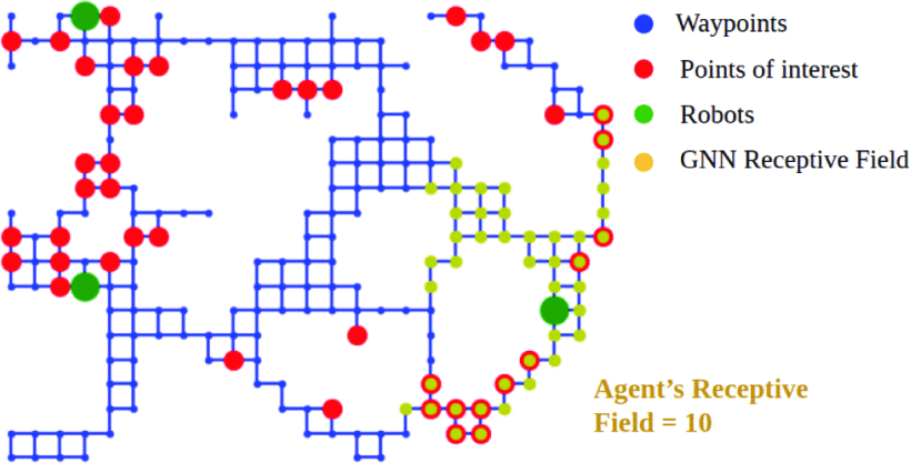
Figure. 3 is the GNN with K=10 visualized during robot training, and green represents the robot being explored. They need to access the red points along the blue waypoints and edge. When the value of k increase, each agent can calculate the controller using information about larger regions of the map [9].
2.6. Baseline controller
We tested the of learning strategies and three different types controllers through experiments. These three controllers are (1) expert open-loop VRP solutions, (2) backward level controllers based on VRP, and (3) greedy controllers. The expert solution is provided by Google's OR Tools library [15]. The expert solution records the length of a task as t, implements the task in an open-loop format, and outputs training data. The planned task length for the horizon controller in reverse is \( \hat{T} \) . And \( T ̂ \lt T \) , it will execute the first step of planning and then replan. The expert controller baseline uses the backward horizontal control shown in Figures 4, 5, and 9[9]. Finally, the greedy controller will use heuristic learning methods to plan each robot to the nearest unexplored waypoint. We use a limited receptive field to achieve planning, using only the K-step distance matrix [9]. We demonstrated this standard in Figures 4, 5, and 9. Because the greedy controller combining limited receptive fields and heuristics is more practical in complex large-scale maps with high computational costs.
2.7. Imitative learning of expert solutions
In imitating the work of experts, we use the stochastic gradient descent to minimize the difference between the actions of experts and the output of the strategy [9], as the space is discrete, there will be cross entropy loss \( L \) :
\( {Π^{*}}=\begin{matrix}ardmin \\ π \\ \end{matrix}\sum _{({G_{t}},{u_{t}})∈D}(π({G_{t}}),{u_{t}})\ \ \ (18) \)
To imitate the strategies of experts, we first need to collect a dataset generated by expert strategy training. In [9], we collect 2000 expert trajectories with a length of \( T \) =50 in random graphs, where \( D={\lbrace ({G_{t}},{u_{t}})\rbrace _{t=1,…,50}} \) . The charts are produced by areas of 228 waypoints from Figure 1 [9]. We test the learning controller on a trajectory with a length \( T \) =50 in the graph generated by the same distribution. These models were trained over 200 periods. The batch size of the training in each training is 32. And we use an Adam optimizer to help the robot train [9].
We use expert controllers to solve exploration problems. The expert controller possesses full graph knowledge and can generate complete trajectory maps. But only retain data on the local state around the robot. The action of the robot will take is based on the observation of the current node and edge and learn by comparing the different behavior between robot and expert. Finally, the robot will perform similar or even identical behavior to the expert controller based on the surrounding environment without full graph knowledge.
3. Results
3.1. Locality
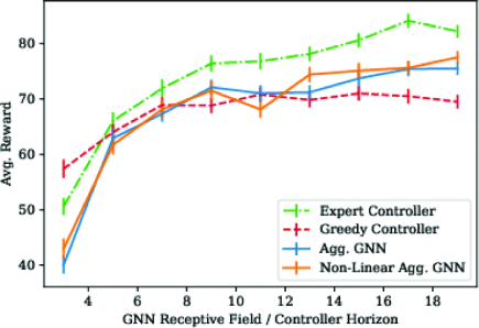
In the coverage task, we made Figures 6. The abscissa represents the receptive field of GNN, and the larger the receptive field, the larger the range of points of interest that the robot can perceive. The ordinate of the graph represents the average reward of the graph. This represents the completion of a coverage task. The higher the average reward, the better the controller completes coverage task. we can conclude from Figure 6 that the GNN controller is significantly better than the greedy controller, but weaker than the expert controller. We can conclude that when the K is low, the performance of GNN controller is improved rapidly when K increase. Linear GNN controller performance is similar to that of non-linear GNN controllers. The open loop expert received the mean reward of 91.0. And the SEM is 0.87 [9]. From the figure, we can conclude that the expert controller can receive the most rewards and have the best performance. The expert controller can provide the upper limit of GNN performance [9].
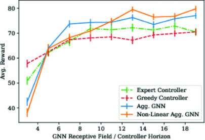
In the exploration task, Figure 7 abscissa and ordinate represent the same meaning as Figure 6. We can conclude from Figure 7 that the performance of the GNN controller is the best, and the performance of expert controller is better than that of greedy controller. The performance of the greedy controller is the worst. For the GNN controller, as the receptive field increases, the performance and the mean reward of the GNN controller also continue to increase.
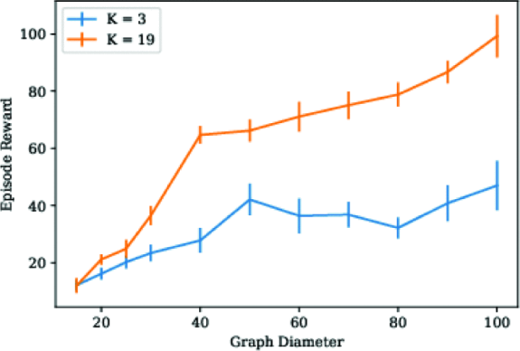
We also tested the effect of different ranges of sensing fields on controller performance and task outcomes under different scale maps. Because the receptive field has a range, we can receive information within that range. We will focus on areas where robots can receive information to solve problem. That will result decentralized solutions [9]. As shown in Figure 5, the robot can only move towards adjacent areas and can only select one area to move at a time. The diameter is the maximum distance between any two nodes [9]. As shown in Figure 10, the performance of models with larger receptive fields is significantly higher than those with smaller receptive fields. And as the diameter of the graph increases, the performance gap between the two controllers will increase. Controllers with larger receptive fields can route proxies to these waypoints. But controllers with smaller receptive field cannot calculate high return paths [9].
|
|
Figure 6. GNNs with a larger receptive field are more likely to achieve higher performance in coverage tasks. The average reward for more than 100 episodes under standard error is displayed [9]. | Figure 7. GNN surpasses expert controllers in exploration tasks. The average reward for more than 100 episodes under standard error is displayed [9]. |
|
|
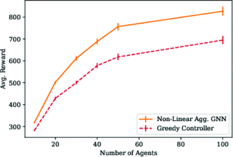
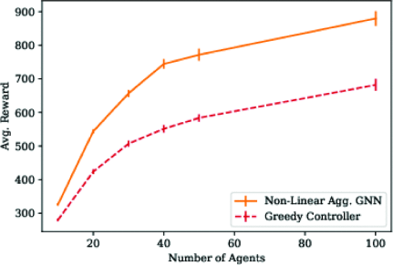
Figure 8. Summary of coverage tasks with 5659 waypoints. We plotted an average reward of over 100 episodes under standard error. [9]. | Figure 9. Summary of exploration tasks with 5659 waypoints. We plotted an average reward of over 100 episodes under standard error. [9]. |
3.2. Transference
We have successfully promoted the GNN model to large robot teams and large maps, which is a scale that traditional VRP solution cannot solve. These models are first trained on 4 agents and an average of 228 waypoints. Then GNN was tested on teams of up to 100 on the map with a size of 5659 waypoints and a diameter of 205[9]. Then we created Figures 8 and Figure 9. The horizontal axis represents the size of the team. Vertical axis represents the completion of the coverage task. The higher the average reward, the better the controller's performance in completing coverage tasks. In Figure 6, we know that the performance of non-linear GNN controller is significantly better than that of greedy controller. In Figure 9, this difference is even greater. We assume that this is because the learning strategy is more capable of learning the weighting of boundary nodes than other unexplored nodes [9].
|
Figure 10. The influence of nonlinear GNN receptive fields in different diameter patterns measured by the average return and standard error of 20 episodes [9]. |
3.3. Dynamics
We successfully use GNN to control coverage missions effectively with ten quadcopter aircraft in large simulation environments, as shown in Figure 1 [9]. A team of 10 robots used a greedy controller and a nonlinear GNN with K=19 for tasks. The team using the greedy controller visited 490 interest points within 400 seconds, while the nonlinear GNN visited 610 interest points. This proves that our graph neural network controller can access more points of interest in the same time for large map and team coverage tasks, and the exploration efficiency of the robot is improved.
4. Conclusion
We apply the GNN method to multi-robot coverage and exploration tasks. This method can extend the coverage task to a team of up to 100 agents, which is difficult for existing expert solutions to achieve. We demonstrate through experiments that the developed graph neural network controller can learn by imitating expert schemes. And after testing, we can conclude that GNN controllers with large receptive fields are significantly better than expert controllers in coverage tasks. In exploration tasks, the GNN controller is significantly superior to the greedy controller. We achieve that the GNN architecture can achieve zero shot generalization for large maps and teams, which is difficult for experts. We also conduct coverage simulation experiments on multi robot teams in urban environments and discuss the dynamic impact of robots during simulation experiments. Otherwise, we demonstrate that our GNN architecture surpasses existing the method based on the planning.
But this paper also has some limitations. The control strategy is only applicable to coverage tasks in some simple environments. In more complex environments or the task on 3D lattices, we may use the on-board sensing strategy. In order to apply GNN to real-world robot teams, we need to consider the issue of two or more robots potentially moving to the same waypoint and causing conflicts. And it is also necessary to achieve collision avoidance function of the robot. We still face many challenges, such as the intermittent communication. In order to solve this challenge, we can allow the robots communicate with each other at regular intervals to update the position, waypoint map, and task progress of other robots. [16] explores a method for implementing data distribution in robot teams.
References
[1]. Zhang H and Hou J C 2005 Maintaining sensing coverage and connectivity in large sensor networks Ad Hoc & Sensor Wireless Networks vol. 1 no. 1-2 pp. 89–124
[2]. Thrun S, Burgard W, and Fox D 2000 A real-time algorithm for mobile robot mapping with applications to multi-robot and 3D mapping Robotics and Automation 2000 Proceedings. ICRA 2000. IEEE International Conference on vol. 1 pp. 321–328
[3]. Thrun S and Liu Y 2005 Multi-robot slam with sparse extended information filers Robotics Research The Eleventh International Symposium. pp. 254–266
[4]. Baxter J , Burke E, Garibaldi J and Norman M 2007 Multi-robot search and rescue: A potential field based approach Autonomous robots and agents. pp. 9–16
[5]. Chen B, Dai B and Song L 2019 Learning to plan via neural explorationexploitation trees arXiv preprint arXiv 1903 00070
[6]. Battaglia P W , Hamrick J B, Bapst V, Sanchez-Gonzalez A, Zambaldi V, Malinowski M, Tacchetti A,Raposo D,Santoro A, Faulkner R et al 2018 Relational inductive biases deep learning and graph networks arXiv preprint arXiv 1806 01261
[7]. Chen F, Bai S, Shan T and Englot B 2019 Self-learning exploration and mapping for mobile robots via deep reinforcement learning AIAA Scitech 2019 Forum p. 0396
[8]. Galceran E and Carreras M 2013 A survey on coverage path planning for robotics Robotics and Autonomous systems vol. 61 no. 12 pp. 1258–1276
[9]. Tolstaya E, Paulos J, Kumar V and Ribeiro A 2021 Multi-Robot coverage and exploration using spatial graph neural networks IEEE/RSJ International Conference on Intelligent Robots and Systems (IROS) Prague Czech Republic pp.8944-8950 doi: 10.1109/IROS51168.2021.9636675
[10]. McNaughton M, Urmson C, Dolan J M, and Lee J W 2011 Motion planning for autonomous driving with a conformal spatiotemporal lattice IEEE International Conference on Robotics and Automation pp. 4889–4895
[11]. Battaglia P W, Hamrick J B, Bapst V, Sanchez-Gonzalez A, Zambaldi V, Malinowski M, Tacchetti A, Raposo D, Santoro A, Faulkner R et al 2018 Relational inductive biases deep learning and graph networks arXiv preprint arXiv:1806.01261
[12]. Kipf T N and Welling M 2017 Semi-supervised classification with graph convolutional networks 5th Int Conf Learning Representations Toulon France Assoc Comput Linguistics 24-26
[13]. Gama F, Marques A G, Leus G and Ribeiro A 2019 Convolutional neural network architectures for signals supported on graphs IEEE Trans. Signal Process vol. 67 no. 4 pp. 1034–1049
[14]. Gama F, Marques A G, Ribeiro A and Leus G 2019 Aggregation graph neural networks 44th IEEE Int. Conf. Acoust., Speech and Signal Process Brighton UK 12-17
[15]. Schulman J, Wolski F, Dhariwal P, Radford A and Klimov O 2017 Proximal policy optimization algorithms arXiv preprint arXiv:1707.06347
[16]. Hill A, Raffin A, Ernestus M, Gleave A, Kanervisto A, Traore R, Dhariwal P, Hesse C, Klimov O, Nichol A, Plappert M, Radford M, Schulman J, Sidor S and Wu Y 2018 Stable baselines https://github. com/hill-a/stable-baselines
Cite this article
Song,M. (2024). Learning based multi-robot coverage algorithm. Applied and Computational Engineering,52,113-122.
Data availability
The datasets used and/or analyzed during the current study will be available from the authors upon reasonable request.
Disclaimer/Publisher's Note
The statements, opinions and data contained in all publications are solely those of the individual author(s) and contributor(s) and not of EWA Publishing and/or the editor(s). EWA Publishing and/or the editor(s) disclaim responsibility for any injury to people or property resulting from any ideas, methods, instructions or products referred to in the content.
About volume
Volume title: Proceedings of the 4th International Conference on Signal Processing and Machine Learning
© 2024 by the author(s). Licensee EWA Publishing, Oxford, UK. This article is an open access article distributed under the terms and
conditions of the Creative Commons Attribution (CC BY) license. Authors who
publish this series agree to the following terms:
1. Authors retain copyright and grant the series right of first publication with the work simultaneously licensed under a Creative Commons
Attribution License that allows others to share the work with an acknowledgment of the work's authorship and initial publication in this
series.
2. Authors are able to enter into separate, additional contractual arrangements for the non-exclusive distribution of the series's published
version of the work (e.g., post it to an institutional repository or publish it in a book), with an acknowledgment of its initial
publication in this series.
3. Authors are permitted and encouraged to post their work online (e.g., in institutional repositories or on their website) prior to and
during the submission process, as it can lead to productive exchanges, as well as earlier and greater citation of published work (See
Open access policy for details).
References
[1]. Zhang H and Hou J C 2005 Maintaining sensing coverage and connectivity in large sensor networks Ad Hoc & Sensor Wireless Networks vol. 1 no. 1-2 pp. 89–124
[2]. Thrun S, Burgard W, and Fox D 2000 A real-time algorithm for mobile robot mapping with applications to multi-robot and 3D mapping Robotics and Automation 2000 Proceedings. ICRA 2000. IEEE International Conference on vol. 1 pp. 321–328
[3]. Thrun S and Liu Y 2005 Multi-robot slam with sparse extended information filers Robotics Research The Eleventh International Symposium. pp. 254–266
[4]. Baxter J , Burke E, Garibaldi J and Norman M 2007 Multi-robot search and rescue: A potential field based approach Autonomous robots and agents. pp. 9–16
[5]. Chen B, Dai B and Song L 2019 Learning to plan via neural explorationexploitation trees arXiv preprint arXiv 1903 00070
[6]. Battaglia P W , Hamrick J B, Bapst V, Sanchez-Gonzalez A, Zambaldi V, Malinowski M, Tacchetti A,Raposo D,Santoro A, Faulkner R et al 2018 Relational inductive biases deep learning and graph networks arXiv preprint arXiv 1806 01261
[7]. Chen F, Bai S, Shan T and Englot B 2019 Self-learning exploration and mapping for mobile robots via deep reinforcement learning AIAA Scitech 2019 Forum p. 0396
[8]. Galceran E and Carreras M 2013 A survey on coverage path planning for robotics Robotics and Autonomous systems vol. 61 no. 12 pp. 1258–1276
[9]. Tolstaya E, Paulos J, Kumar V and Ribeiro A 2021 Multi-Robot coverage and exploration using spatial graph neural networks IEEE/RSJ International Conference on Intelligent Robots and Systems (IROS) Prague Czech Republic pp.8944-8950 doi: 10.1109/IROS51168.2021.9636675
[10]. McNaughton M, Urmson C, Dolan J M, and Lee J W 2011 Motion planning for autonomous driving with a conformal spatiotemporal lattice IEEE International Conference on Robotics and Automation pp. 4889–4895
[11]. Battaglia P W, Hamrick J B, Bapst V, Sanchez-Gonzalez A, Zambaldi V, Malinowski M, Tacchetti A, Raposo D, Santoro A, Faulkner R et al 2018 Relational inductive biases deep learning and graph networks arXiv preprint arXiv:1806.01261
[12]. Kipf T N and Welling M 2017 Semi-supervised classification with graph convolutional networks 5th Int Conf Learning Representations Toulon France Assoc Comput Linguistics 24-26
[13]. Gama F, Marques A G, Leus G and Ribeiro A 2019 Convolutional neural network architectures for signals supported on graphs IEEE Trans. Signal Process vol. 67 no. 4 pp. 1034–1049
[14]. Gama F, Marques A G, Ribeiro A and Leus G 2019 Aggregation graph neural networks 44th IEEE Int. Conf. Acoust., Speech and Signal Process Brighton UK 12-17
[15]. Schulman J, Wolski F, Dhariwal P, Radford A and Klimov O 2017 Proximal policy optimization algorithms arXiv preprint arXiv:1707.06347
[16]. Hill A, Raffin A, Ernestus M, Gleave A, Kanervisto A, Traore R, Dhariwal P, Hesse C, Klimov O, Nichol A, Plappert M, Radford M, Schulman J, Sidor S and Wu Y 2018 Stable baselines https://github. com/hill-a/stable-baselines