1. Introduction

1.1. Research Background

Array signal processing is extremely widely applied in many fields, such as wireless communications, radar, etc. The problems studied in array signal processing include beamforming techniques, spatial spectrum estimation, source localization, and source separation [1]. Among these, the issues with beamforming techniques involve the process of receiving signals through an array of beam sensors and processing them, known as space principle production or Direction of Arrival (DOA) estimation, to achieve super-resolution estimation of the propagation direction distribution of multiple signal waves in space. The main goals of spatial spectrum estimation research include algorithm design and optimization, array structure design and optimization, aiming for algorithms with high accuracy and low complexity, straightforward design structures, and arrays with a high degree of freedom (DOF).

1.2. Current Research Status

The Multiple Signal Classification (MUSIC) algorithm was first proposed by Schmidt in 1979 [2], significantly advancing the field of array signal processing research. Barabel later introduced the one-dimensional root-MUSIC algorithm, which replaced the traditional peak searching process with polynomial rooting, successfully reducing computational complexity. The classic two-dimensional MUSIC algorithm was first presented by WAX and his colleagues in 1984 [3]. Roy and others proposed the signal parameter estimation method using rotation invariant techniques [4], differentiating technologically. This algorithm was developed in response to scenarios where the signal source and the sensor array are not coplanar, introducing a progressive, unbiased, one-dimensional direction cosine estimation algorithm. Additionally, research has utilized non-uniform arrays in multi-target parameter estimation for MIMO radars, further enhancing the degrees of freedom and estimation accuracy of the radar system. DOA estimation methods in non-uniform arrays have been extensively studied, with traditional super-resolution algorithms being deeply explored, especially for one-dimensional DOA estimation methods. Algorithms like MUSIC, ESPRIT, and their related methods have been widely applied. Beyond studying DOA algorithms, the design and optimization of array structures also require attention. Although the physical structure of uniform linear arrays is simple, they can only perform one-dimensional azimuthal angle estimation since each element is on a straight line. Many scholars have also proposed L-shaped arrays [5], planar arrays [6], and uniform circular arrays [7] for implementing two-dimensional angle estimation.

While traditional arrays are effective for DOA estimation, they have a drawback: the array's degrees of freedom are limited, only able to detect a number of signal sources equivalent to the number of array elements. In early research on the problem of direction cosine estimation when the number of signal sources exceeds the number of array elements, many different solutions were proposed. An important research topic in Multi-Input Multi-Output (MIMO) radar in recent years is the DOA estimation problem, with relevant research findings emerging in large quantities. The Reduced-Dimension (RD) ESPRIT algorithm, used for estimating the direction angle in single-antenna MIMO radar, aims to reduce dimensions through the ESPRIT algorithm, thus lowering the algorithm's computational complexity. The Real-valued ESPRIT algorithm first performs dimensionality reduction for non-circular signals, then uses a matrix to convert signal information into real numbers, further reducing computational complexity. This algorithm is mainly used for estimating the incidence angle of one-dimensional signals, while it cannot be applied for two-dimensional signal incidence angles. In recent years, sparse array parameter estimation technology has been introduced to MIMO radar systems. Compared to traditional MIMO radar, sparse MIMO radar can increase the array's degrees of freedom. Combining nested matrices in sparse matrices with MIMO radar can maximize the utilization of the relationship between transmission and reception matrices, thus maintaining the effective degrees of freedom of MIMO radar and enhancing angular estimation performance.

2. Spatial Smoothing MUSIC Algorithm

2.1. Principle of the MUSIC Algorithm

When the received signal is a narrowband signal, taking a linear antenna array as an example, with K = 1, 2, ..., denoting the sequence, the signals injected into the antenna array are \( θk \) , k, as shown in Figure 1, with M antennas having an element spacing of D. It is assumed that the signal vector S(N) is incident on the antenna array:

s(n) = ( \( s1 \) (n) , \( s2 \) (n) ,… \( sK \) (n) )

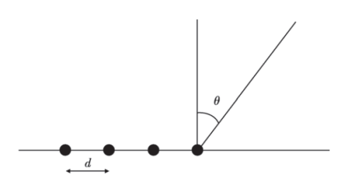
Figure 1. M antennas with an element spacing of D

The array response vector of a uniform linear array is:

\( a(θk)=[1,exp{(}-2Π\frac{d}{λ}sin{θ}k) \) \( exp{[}-2Π(M-1)\frac{d}{λ}sin{θ}k)] \)

The direction matrix is \( A=[a(θ1),a(θ2),...,a(θk)] \) , and all signals incident on the antenna array units summed together can form a received signal: \( x(n)=a(θ1)s1(n)+...a(θk)sk(n) \) . Due to additive noise in the real environment, the received signal array is represented as follows: \( x(n)=As(n)+v(n) \) . The data vector received by this array is x(n), the array direction matrix is a, the spatial signal vector is s(n), and the white noise vector is v(n). The spatial correlation matrix can be represented by the following equation for the received signal vector: \( R=E[x(n){x^{H}}(n)]=ARs{A^{H}}+{σ^{2}}I \) .

2.2. Simulation Analysis of the MUSIC Algorithm

Initially, three incoherent signal sources are simulated using MATLAB, further simulating the MUSIC algorithm with an 8-antenna segment. The MUSIC direction-finding results are given in MATLAB simulations, as shown in Figures 2 and 3.

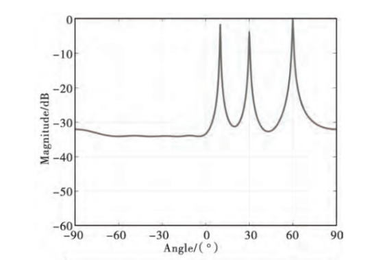
Figure 2. MUSIC direction-finding results for a 10° direction signal source

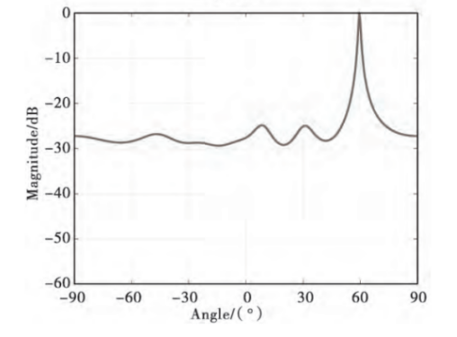
Figure 3. MUSIC direction-finding results for a 30° direction signal source

The signal sources in the figures include three mutually incoherent signal sources, with the top images representing signal sources at 10° and 30° directions, respectively. According to the simulation results, we know that the MUSIC algorithm can effectively distinguish incoherent signal sources in the measured direction, but it cannot effectively distinguish coherent signal sources in the measured direction [8].

3. Spatial Smoothing PM Algorithm

3.1. Principle of the PM Algorithm

Similar to the SS-MUSIC algorithm, in the Spatial Smoothing PM (SS-PM) algorithm, the process of spatial smoothing involves dividing the truncated virtual array into Mn+1 overlapping sub-arrays, each containing Mn+1 elements. The average of all Mn+1 sub-array covariance matrices is computed to calculate the received signal of the sub-array covariance matrices, including Mn+1 sub-arrays, to obtain the Spatial Smoothing Covariance Matrix R(SpaceComplexMatrixr), which is in the same format as the signal covariance matrix, based on classical subspace algorithms. The DOA estimates of spatial sources will be obtained by the classical PM algorithm applying to MatrixR as follows.

Similar to the ESPRIT algorithm, the PM algorithm is also based on array rotation, rather than relying on it. Since the virtualization of augmented coprime linear arrays produces a virtual uniform linear array, we briefly introduce the principle of the PM algorithm based on uniform linear arrays below.

Considering there are K signals, with their direction of arrival angles on a uniform linear array, the direction matrix of the array (with M elements and N sources) can be divided into a block containing M elements with an element spacing of D. \( θ1θ2θk \) : \( A=[\begin{matrix}A1 \\ A2 \\ \end{matrix}] \) , \( A∈{C^{M×K}} \)

It includes a full rank matrix (fullmatrix) between two moment matrices, with a linear propagation operator that makes the estimate as: ( \( A1∈{C^{K×K}} \) , \( A2∈{C^{(M-N)×K}} \) , \( PC∈{C^{(M-N)×K}} \) ) \( PC=[{G^{+}}H{]^{H}} \)

Defining matrix \( P∈{C^{M×K}} \) as: \( P=[\begin{matrix}IK \\ PC \\ \end{matrix}] \) then the direction matrix A can be expressed as: \( A=[\begin{matrix}A1 \\ A2 \\ \end{matrix}]=PA1 \)

Let \( Pa \) and \( Pb \) represent the first M-1 rows and the last M-1 rows of matrix P, respectively, and let \( Aa \) and \( Ab \) represent the first M-1 rows and the last M-1 rows of matrix A, respectively. Then: \( [\begin{matrix}Pa \\ Pb \\ \end{matrix}]A1=[\begin{matrix}Aa \\ Ab \\ \end{matrix}]=[\begin{matrix}Aa \\ Aaφr \\ \end{matrix}] \) , it follows that: \( P{a^{+}}Pb=A1φrA{1^{-1}} \)

Defined as follows: The Direction of Arrival (DOA) estimates of the sources can be obtained through the eigen decomposition of the signal matrix. \( φr=P{a^{+}}Pb \)

3.2. Algorithm Effectiveness Verification

To validate the effectiveness of the algorithm and describe its angle estimation performance, this section utilizes Montecarlo simulations with 1000 iterations. Considering K=13 uncorrelated narrowband signals incident on an augmented coprime linear array with M=4, N=5, uniformly distributed across azimuth angles from -60° to 60°, J=500, SNR=5dB. Figure 4 shows the estimation results of the SS-PM algorithm. The figure demonstrates that the SS-PM algorithm can effectively estimate the angles of signal sources, capable of estimating more signal sources than the actual number of array elements.

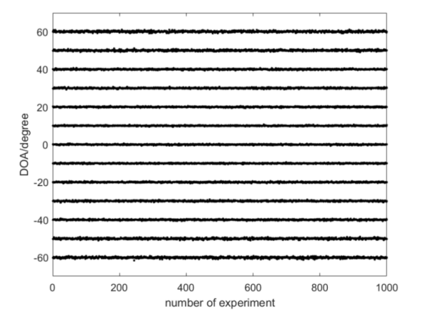
Figure 4. Estimation Results of the SS-PM Algorithm

4. DOA Estimation Based on Spatial Smoothing MUSIC Algorithm

To precisely evaluate the performance of the algorithm, multiple experiments are necessary to assess its angular estimation accuracy accurately. We use the Root Mean Square Error (RMSE) to define the accuracy of angle estimation during these evaluations:

\( RMSE=\frac{1}{K}\begin{matrix}K \\ a \\ k=1 \\ \end{matrix}\sqrt[]{\frac{1}{J}\begin{matrix}J \\ a \\ j=1 \\ \end{matrix}[(qk,j-qk{)^{2}}]} \)

Here, K is the number of signal sources, \( qk,j \) is the estimated angle of the k-th signal source in the j-th simulation, and \( qk \) is the actual angle of the k-th signal source. J is the number of simulations, and for the simulations below, we take J=500 [9].

Assume an incoherent signal source, with its angles of incidence, injected into the far-field space of a nested array. \( KM,qk(k=1,2,L,K) \) are the number of elements, with L being the number of snapshots.

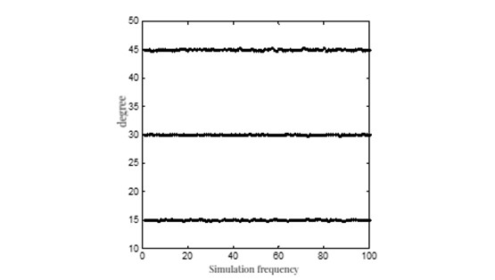
Simulation 1. In this section, we obtained scatter plots of the angle of incidence estimates of one-dimensional signals under definite conditions, using simulation techniques. During simulation, we used a search step size of 0.01. The algorithm studied can accurately estimate the angles of incidence based on Figure 5. (K<M)

\( θ=[-50°,-35°,-10°,0°,15°,30°,45°,55°,70°],K=9,SNR=-5dB,M=8,L=600 \)

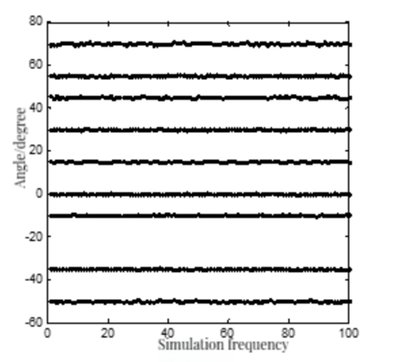
Simulation 2. This part simulates the one-dimensional DOA estimation graph of the studied algorithm under indefinite conditions. The algorithm, as observed in Figure 6, can accurately estimate the angles of incidence when the number of signal sources exceeds the number of antenna elements [10].

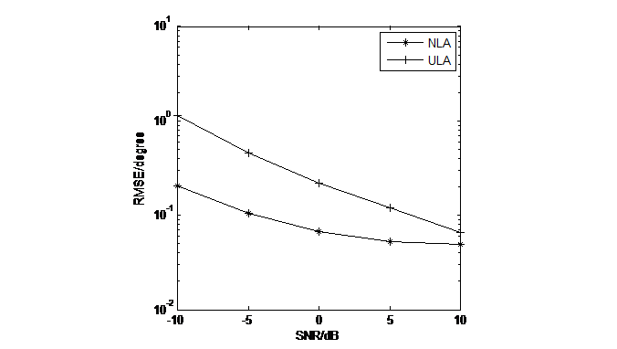
Simulation 3. In this section, we simulated and compared the performance between the studied algorithm in one-dimensional Direction of Arrival (DOA) estimation and the traditional Uniform Line Array (ULA) MUSIC algorithm. A search step size of 0.01 was set for the simulation. From Figure 7, it is clear that, performance-wise, the studied algorithm outperforms the ULA MUSIC algorithm. This section studied the Spatial Smoothing MUSIC algorithm under Nested Arrays, abbreviated as NLA, with the traditional calculation for the uniform line array as ULA. \( q1=15°,q2=30°,q3=45°,M=8,L=600 \)

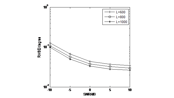
This section compared one-dimensional DOA estimation performances with different sampling rates. The search step size during the simulation was 0.01. The studied algorithm's angle estimation accuracy improves with the increase in the number of snapshots, as clearly observed in Figure 8. \( L=600,L=800,L=1000,q1=30°,q2=30°,q3=45°,M=8 \)

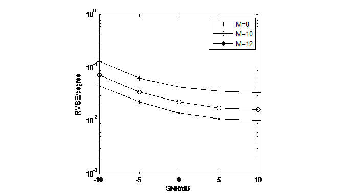
Simulation 5. Performance comparison of DOA estimation values under different arrays is the focus of this section. The simulation search step size was 0.01. From Figure 9, we can see that the studied algorithm's angle estimation performs better when the number of elements increases. \( M=6,M=8,M=10,q1=15°,q2=30°,q3=45°,L=600 \)

5. Performance Analysis

5.1. Degrees of Freedom

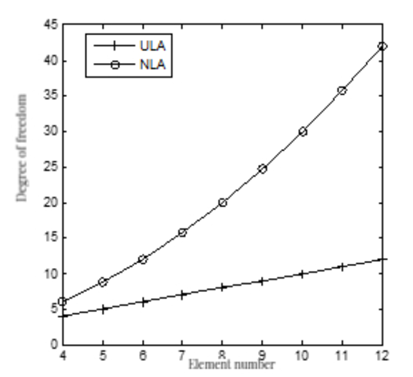
This section compares the degrees of freedom (DOF) between nested array structures and uniform linear array structures under the same physical element conditions. The DOF of a nested array structure is given by \( DOF=\frac{N+1}{2} \) , whereas for a uniform linear array structure \( DOF=M \) , where M denotes the number of elements, and \( N=({M^{2}}/2+2M-2)/2 \) [11].

Figure 10 displays the comparison of available degrees of freedom between nested array structures and uniform linear arrays, where ULA represents the uniform linear array, and NLA represents the nested array, when the number of elements is given. As seen from the figure, the available degrees of freedom for nested arrays are much greater than those for uniform linear arrays.

5.2. Summary of Algorithm Advantages

The main advantages of the studied algorithm can be summarized as follows:

1) The algorithm discussed in this section can be used for undetermined DOA estimation values; K>M

2) The spatial smoothing MUSIC algorithm for nested arrays offers higher available degrees of freedom than uniform linear arrays under the same physical sensor layout.

3) The angle estimation performance of the studied algorithm is better than that of the traditional uniform linear array (ULA) MUSIC algorithm under the same physical element conditions.

6. Conclusion

This paper primarily investigated the spatial smoothing MUSIC algorithm for nested arrays. Such algorithms, through a special arrangement, enhance the array's degrees of freedom and resolution, thus enabling the processing of more signal sources. Compared to uniform linear array algorithms, this class of algorithms significantly improves angle estimation performance and can handle source estimation under undetermined conditions. The angle estimation of the studied algorithm performs better than the traditional uniform linear array (ULA) MUSIC algorithm under the same physical element conditions.

References

[1]. Krim H, Viberg M. Two decades of array signal processing research: the parametric approach[J]. IEEE Signal Processing Magazine, 1996, 13(4): 67-94.
[2]. Schmidt R O. Multiple emitter location and signal parameter estimation[J]. IEEE Transactions on Antennas and Propagation, 1986, 34(3): 276-280.
[3]. Wax M, Shan T J, Kailath T. Spatial-temporal spectral analysis by eigenstructure method[J]. IEEE Transactions on Acoustics Speech and Signal Processing, 1984, 32(4): 817-827.
[4]. Roy R, Kailath T. ESPRIT-estimation of signal parameters via rotational invariance techniques[J]. IEEE Transactions on Acoustics Speech and Signal Processing, 1989, 37(7):984-995.
[5]. Hua Y, Sarkar T K, Weiner D D. An L-shaped array for estimation 2-D directions of wave arrival[J]. IEEE Transactions on Antennas and Propagation, 1991, 39(2): 143-146
[6]. Zoltowski M D, Haardt M, Mathews C P. Closed-form 2-D angle estimation with rectangular arrays in element space or beamspace via unitary ESPRIT[J]. IEEE Transactions on Signal Processing, 1996, 44(2): 316-328.
[7]. Wang, D., & Wu, Y. (2006). Research on two-dimensional ESPRIT algorithm based on uniform circular array. Journal of Communications, (9), 89-95.
[8]. Zheng, C., & Yang, Z. Q. (2021). Coherent source DOA of the spatial smoothing MUSIC algorithm. Fire Control Radar Technology, 50(03), 21-24. DOI:10.19472/j.cnki.1008-8652.2021.03.005.
[9]. Li, J. H., Yang, Z. Q., & Hua, L. (2022). Research on DOA spatial spectrum estimation of coherent sources. Fire Control Radar Technology, 51(02), 28-31. DOI:10.19472/j.cnki.1008-8652.2022.02.005.
[10]. Ai, M., Yu, G. C., & Wang, Z. Q. (2019). DOA estimation algorithm for interpolated array elements in coprime array apertures. Journal of Nanchang University (Engineering Edition), 41(04), 398-403. DOI:10.13764/j.cnki.ncdg.2019.04.015.
[11]. Zhang, X. F., Chen, H. W., Qiu, X. F., et al. (2015). Array Signal Processing and MATLAB Implementation. Beijing: Electronics Industry Press.
Cite this article
Sun,M.;Duanmu,T. (2024). DOA estimation technology based on array signal processing nested array. Applied and Computational Engineering,64,23-29.
Data availability
The datasets used and/or analyzed during the current study will be available from the authors upon reasonable request.
Disclaimer/Publisher's Note
The statements, opinions and data contained in all publications are solely those of the individual author(s) and contributor(s) and not of EWA Publishing and/or the editor(s). EWA Publishing and/or the editor(s) disclaim responsibility for any injury to people or property resulting from any ideas, methods, instructions or products referred to in the content.
About volume
Volume title: Proceedings of the 6th International Conference on Computing and Data Science
© 2024 by the author(s). Licensee EWA Publishing, Oxford, UK. This article is an open access article distributed under the terms and
conditions of the Creative Commons Attribution (CC BY) license. Authors who
publish this series agree to the following terms:
1. Authors retain copyright and grant the series right of first publication with the work simultaneously licensed under a Creative Commons
Attribution License that allows others to share the work with an acknowledgment of the work's authorship and initial publication in this
series.
2. Authors are able to enter into separate, additional contractual arrangements for the non-exclusive distribution of the series's published
version of the work (e.g., post it to an institutional repository or publish it in a book), with an acknowledgment of its initial
publication in this series.
3. Authors are permitted and encouraged to post their work online (e.g., in institutional repositories or on their website) prior to and
during the submission process, as it can lead to productive exchanges, as well as earlier and greater citation of published work (See
Open access policy for details).