1. Introduction

1.1. Motivation

Prostate diseases are a group of ailments that affect the prostate gland in men, the most prevalent of which are prostatitis, benign prostatic hyperplasia (BPH), and prostate cancer. These diseases cause significant harm to human health and highlight the necessity of early detection for successful management and treatment [1]. They can have a variety of negative repercussions on people, including physical, emotional, and social consequences. For starters, they can induce urinary symptoms such as frequent urination, urgency, weak urine flow, and incomplete bladder emptying, disturbing everyday activities and lowering quality of life. Persistent or severe symptoms might also cause sleep difficulties, persistent discomfort, and psychological suffering.

Prostate illnesses cause substantial harm to individuals and can lead to consequences if left undetected or untreated. Early diagnosis is critical for limiting detrimental consequences, improving outcomes, and decreasing the burden on individuals and society.

1.2. Problem definition

In order to assist doctors in early diagnosis of prostate diseases and improve the accuracy of early diagnosis, the author has chosen to use machine learning to establish an early prostate disease screening and prediction model.

By training the existing data sets and establishing the machine learning model, the possibility of prostate cancer and benign prostatic hyperplasia can be predicted by evaluating a series of medical test indexes of patients.

2. Methodology

2.1. Logistic regression

Predictive analytics and classification frequently employ this kind of statistical model called logit model. The logistic function can also be expressed as the natural logarithm of odds or log odds. These formulae are used to describe the logistic function:

\( Logit({p_{i}})=\frac{1}{1+{e^{-{p_{i}}}}} \)

\( ln{(\frac{{p_{i}}}{1-{p_{i}}})}={β_{0}}+{x_{1}}{β_{1}}+…+{x_{n}}{β_{n}} \)

In this logistic regression equation, x is the independent variable and logit(pi) is the dependent variable, also known as the response variable. The beta parameter, or coefficient, in this model is often estimated using maximum likelihood estimation (MLE). This method continuously assesses several values of beta in order to optimize for the best fit of log odds. Logistic regression optimizes the log likelihood function—the outcome of all these repetitions—to obtain the best estimate of the parameter. When the best coefficient—or coefficients, if there are numerous independent variables—is found, the conditional probabilities for each observation can be computed, logged, and summed together to yield a predicted probability. The procedure of evaluating the how well the model predicts the dependent variable is called goodness of fit [3].

2.2. Naive Bayes

Given that it is based on Bayes' Theorem, Naive Bayes is frequently referred to as a probabilistic classifier. Without first going over the fundamentals of Bayesian statistics, it would be challenging to describe this method. Conditional probabilities can be inverted according to this theorem, which is sometimes referred to as Bayes' Rule [2]. Recall that conditional probabilities are the likelihood of an event given the occurrence of another event. This may be expressed using the following formula:

\( P(Y|X)=\frac{P(X and Y)}{P(X)} \)

The Bayes’ Theorem is unique in that it applies to sequential occurrences, in which the starting probability is affected by subsequently obtained information. The posterior probability and the prior probability are the names given to these probabilities [4]. The initial likelihood of an occurrence before it is contextualized within a certain scenario is known as the prior probability, also known as the marginal probability. The likelihood of an event occurring after viewing certain data is known as the posterior probability.

2.3. Decision trees

A decision tree is a non-parametric supervised learning algorithm, which is utilized for both classification and regression tasks. Its internal nodes, leaf nodes, branches, and root node make up its hierarchical tree structure. With no incoming branches, a decision tree begins with a root node. The internal nodes—also referred to as decision nodes—are fed by the outgoing branches that originate from the root node. Leaf nodes and terminal nodes are examples of homogeneous subsets formed by evaluations conducted by both node types based on available attributes. All of the possible outcomes in the dataset are represented by the leaf nodes.

In order to find the best split points inside a tree, decision tree learning uses a divide and conquer tactic by searching greedily. After that, the splitting procedure is repeated in a top-down, recursive fashion until all or most records are assigned a specific class label [5]. Pruning, which involves removing branches that split on traits of low value, is typically used to minimize complexity and prevent overfitting. Then, using the cross-validation procedure, the model's fit may be assessed.

2.4. Random Forest

By combining feature randomness with bagging, the random forest algorithm builds an uncorrelated forest of decision trees, which is an extension of the bagging technique. Feature randomness—also referred to as "the random subspace method" or feature bagging—produces a random selection of features that guarantees low correlation between decision trees. One of the main distinctions between random forests and decision trees is this [6]. Random forests choose only a portion of the characteristics that can divide, whereas decision trees take into account all possible splits. Predictions can be made more precisely by taking into account all possible variability in the data, which also lowers the danger of overfitting, bias, and overall variance.

2.5. K-nearest Neighbors Algorithm

2.5.1. Brief introduction

The K-nearest Neighbors Algorithm, sometimes referred to as KNN or k-NN, is a non-parametric supervised learning classifier that makes predictions or classifications about how to categorize a single data point based on its proximity. It is usually employed as a classification algorithm, based on the idea that comparable points can be discovered close to one another, though it can be used for regression or classification problems as well [7].

When it comes to classification challenges, the label that is most commonly expressed around a particular data point is utilized to assign a class label based on a majority vote.

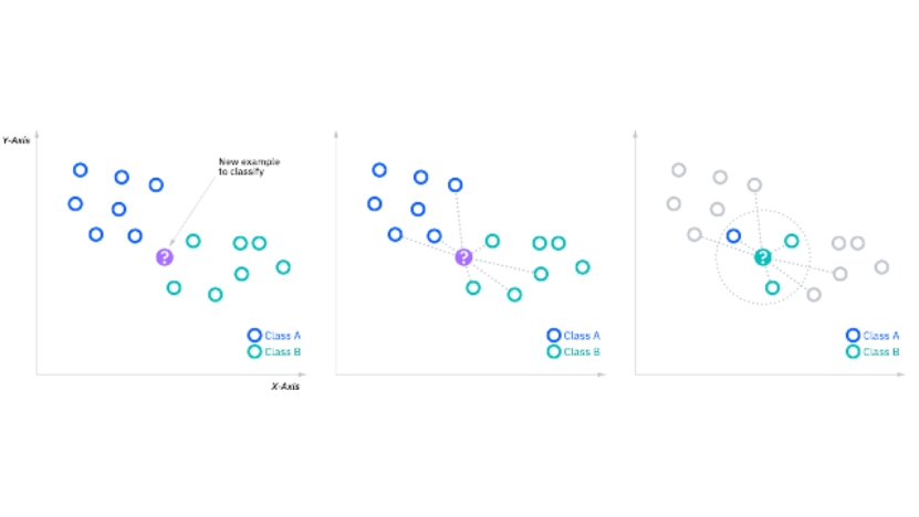
Figure 1. A simple data set classified by the KNN algorithm

The k-nearest neighbor algorithm seeks to locate a query point's closest neighbors so that a class label can be applied to it. KNN needs to meet a few prerequisites in order to perform this:

2.5.2. Determine the distance metrics

It is necessary to compute the distance between a query point and all other data points in order to ascertain which data points are closest to a particular query point. By dividing query points into several regions, these distance metrics aid in the formation of decision boundaries [8]. There are many different distance metrics available, but only the following will be discussed in this article:

2.5.3. Euclidean distance (p=2)

\( d(x,y)=\sqrt[]{\sum _{i=1}^{n}{({y_{i}}-{x_{i}})^{2}}} \)

2.5.4. Manhattan distance (p=1)

\( d(x,y)=\sum _{i=1}^{m}|{x_{i}}-{y_{i}}| \)

2.5.5. Minkowski distance

\( d(x,y)={(\sum _{i=1}^{m}|{x_{i}}-{y_{i}}|)^{\frac{1}{p}}} \)

2.5.6. Hamming distance

2.5.1 \( d(x,y)=\sum _{i=1}^{k}|{x_{i}}-{y_{i}}| \)

\( x=y D=0 \)

\( x≠y D≠1 \)

2.5.7. Compute KNN: defining k

In the k-NN algorithm, the k parameter indicates the number of neighbors that will be examined in order to classify a given query point. If k equals 1, for instance, the instance will belong to the same class as its closest neighbor. Different values can result in either overfitting or underfitting, therefore defining k can require some balancing. Higher values of k may result in reduced variance and higher bias, while lower values may have low bias and higher variance. Data with more noise or outliers will probably perform better with higher values of k, therefore the choice of k will mostly depend on the input data.

2.6. Support vector machines

For regression or classification, SVMs are a well-liked supervised learning model. When applied to small data sets, this method is efficient in high-dimensional spaces (many features in the feature vector). After been trained on a set of data, the system can effectively identify fresh observations with ease. To do this, it divides the data set into two classes using one or more hyperplanes [9].

2.7. XGBoost

A scalable, distributed machine learning framework for gradient-boosted decision trees (GBDTs) is called Extreme Gradient Boosting, or XGBoost. With parallel tree boosting, it is the best machine learning software for problems with regression, classification, and ranking [10].

The intrinsic interpretability of decision trees is lost in the process, even if the XGBoost model often beats a single decision tree in terms of accuracy. It is easy to follow the course of a decision tree, for example, but harder to trace the paths of hundreds or thousands of trees [11].

2.8. The ROC (Receiver Operating Characteristic)

One visual method for assessing how well categorization models work is the Receiver Operating Characteristic (ROC) curve. It displays the classification model's performance at various classification thresholds by plotting the false positive rate (FPR) on the x-axis and the true positive rate (TPR), also referred to as sensitivity or recall [12].

The ROC curve has several advantages:

• Intuitiveness: The ROC curve provides an intuitive visualization of the classification model's performance at different classification thresholds. The shape and slope of the ROC curve can be used to judge the model's effectiveness.

• Robustness: The ROC curve is robust to class imbalance and incorrectly classified samples, making it a better choice for evaluating classification model performance.

• Comparative analysis: The ROC curve is not affected by the classification threshold, making it suitable for comparing different models. By comparing the ROC curves of different models, the best performing model can be selected.

• Interpretation: The ROC curve can comprehensively evaluate the performance of the classification model for different data distributions and visualize the mistakes made by the classifier.

The ROC curve is an intuitive and effective graphical tool for evaluating classification model performance. Its advantages include interpretability, robustness to data imbalance, comparability, and robustness. Using the ROC curve in evaluating classification models can provide a more comprehensive understanding of model performance and comparison between different models.

2.9. Cross-validation

Cross-validation is a statistical concept used to evaluate the performance of machine learning models. This process involves dividing the dataset into "training sets" and "validation sets" and iterating between them to ensure the model's predictive ability while expanding its experience [13].

2.9.1. The steps of cross-validation are as follows:

• The dataset is split into k smaller subsets, also known as "folds".

• For each specific fold, the model is first trained using the data from the other k-1 folds, and then the performance of the model is evaluated using this specific fold.

• This process is repeated k times, with each iteration selecting a different fold for validation and the remaining folds for training.

• Finally, k models and their respective validation results can be obtained, typically averaging the results to evaluate the overall model performance.

2.9.2. The main advantages of cross-validation are:

• Model robustness: Cross-validation provides more confidence in a model's performance on unseen data by training and evaluating it on different training and validation sets. This process helps improve model robustness and prevent overfitting.

• Model evaluation: Cross-validation allows you to make better use of all available data to build and evaluate models, avoiding the waste of data that occurs with a single split.

• Parameter tuning: Cross-validation is an excellent tool for model tuning. When trying different parameter settings, such as regularization parameters and learning rates, cross-validation helps understand which combinations provide the best predictive performance.

• Overall, cross-validation is a valuable technique for assessing and improving model performance in machine learning [14].

3. Experiment

The dataset is from China National Population Health Science Data Center which released the prostate early warning data set. And Jupyter Notebook is used as the IDE.

The first part is to evaluate the whole dataset. By applying the Profile Report function, the basic features of the dataset are shown as follows.

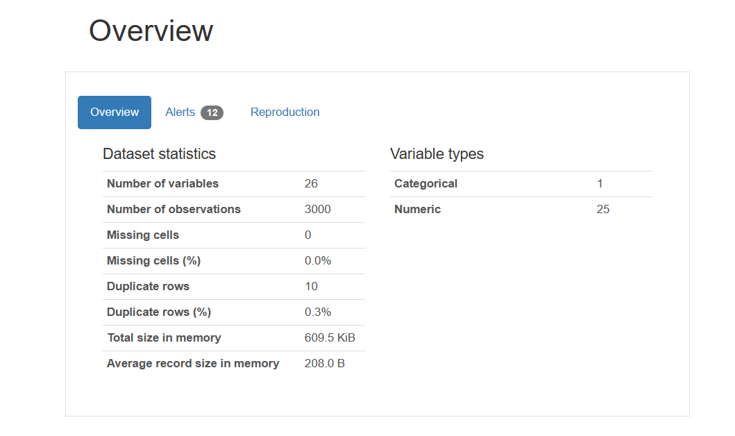
Figure 2. An overview of the dataset

Here plots a bar chart displaying the frequency of prostate cancer and prostate hyperplasia. It uses the pd.cut() function to divide the Age column into 10 intervals and create a new column named 'age_cat'. Then, it uses the pd.crosstab() function to create a cross-tabulation, calculating the frequency of prostate cancer and hyperplasia for each age group. Next, the plot() function is used to create the bar chart, and various properties such as the title, axis labels, tick labels, and legend are set. Finally, the chart is displayed.

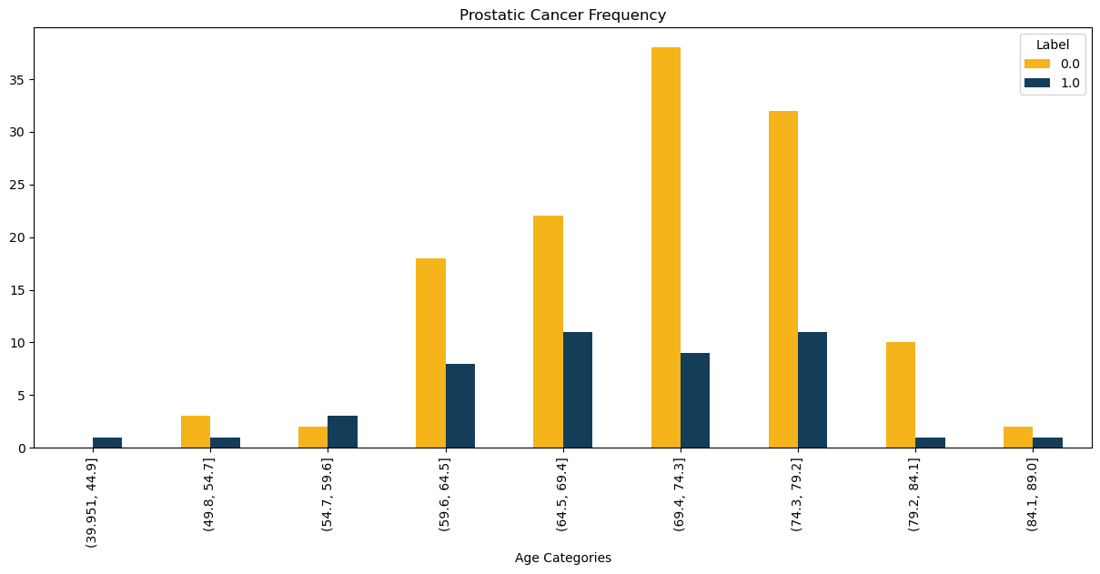
Figure 3. Sample output

The next step is to standardize the data. Here is the result.

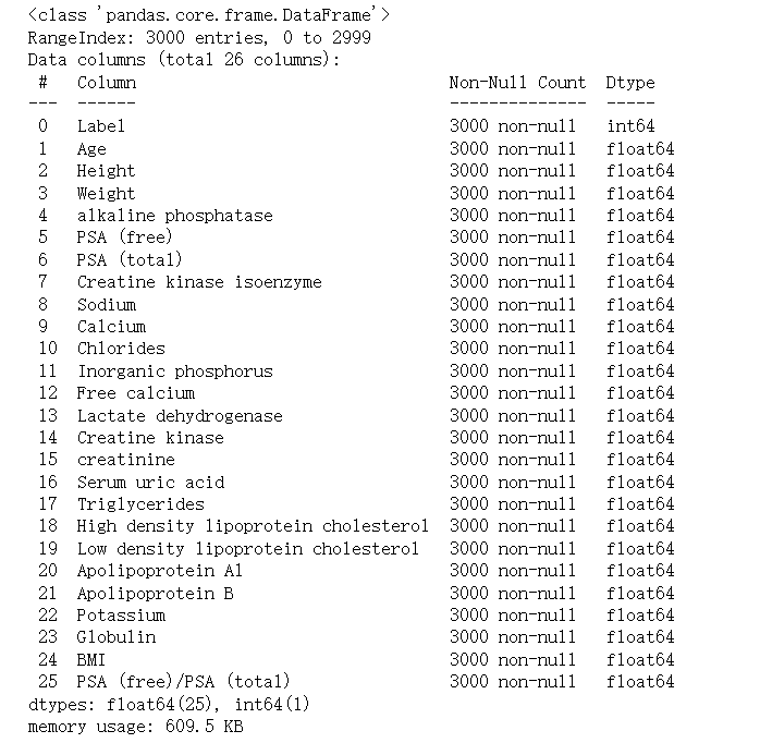
Figure 4. Sample output

Here is the result of logistic regression.

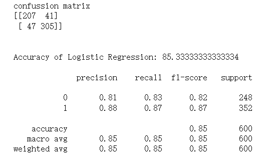
Figure 5. Sample output

Here is the result of random forest classifier.

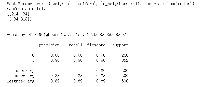
Figure 6. Sample output

Here is the result of XGBoost.

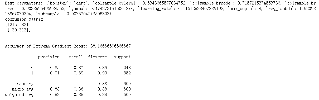
Figure 7. Sample output

Here is the result of decision tree.

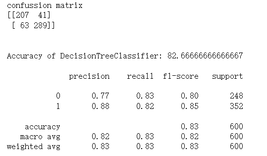
Figure 8. Sample output

Here is the result of support vector classifier.

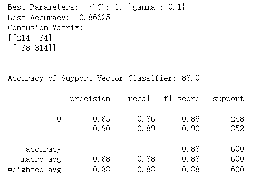
Figure 9. Sample output

Here is the result of naïve bayes.

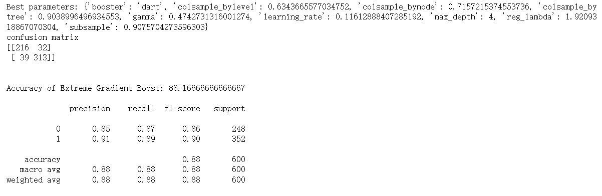
Figure 10. Sample output

It is vital to visually represent the feature importance, allowing for a more intuitive understanding of the importance of each feature in the model. Here is the bat plot.

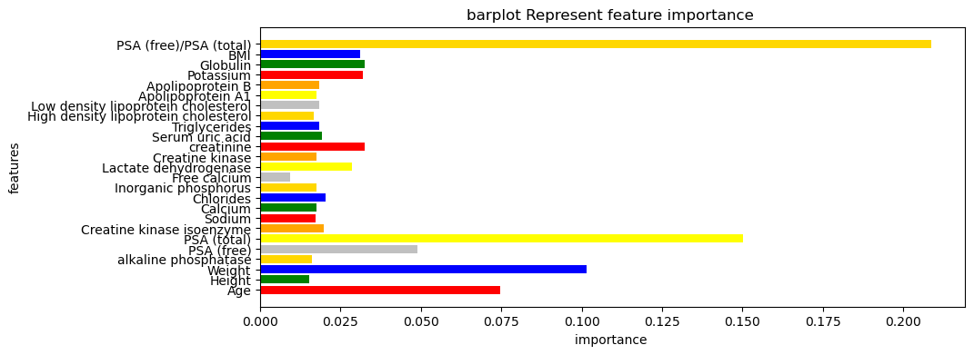
Figure 11. Bar plot of the feature importance

Here is the ROC (Receiver Operating Characteristic) curve.

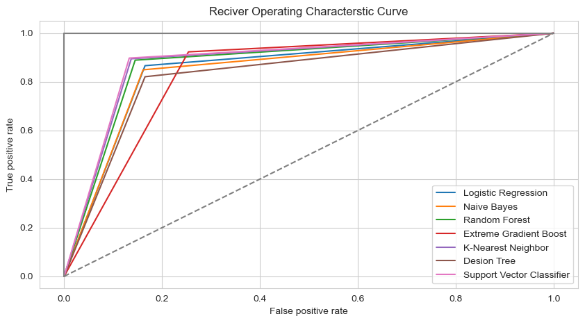
Figure 12. ROC curve

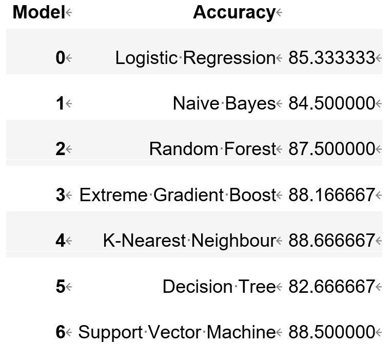
Figure 13. Result

The last part of the experiment is to apply the ensemble model. StackingCVClassifier model from the mlxtend library is applied, which is a stacked generalization model based on cross-validation. It specified multiple base classifiers, including svc, knn, and rf, using the classifiers parameter. It also specified a meta-classifier, svc, to integrate the predictions from the base classifiers.

The model is trained by using the fit() method and made predictions on the X_test data using the predict() method. the confusion matrix, conf_matrix, and accuracy score, acc_score, using confusion_matrix() and accuracy_score() functions are computed, respectively. Finally, it printed the confusion matrix and accuracy score, and used the classification_report() method to output a detailed classification report of the predicted results.

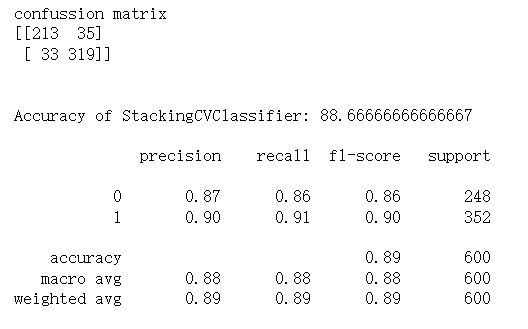
Figure 14. result after applying ensemble model

4. Conclusion

4.1. Generalization

Various machine learning methods were applied to train the data. Finally, it is found that Support Vector Machine has the highest accuracy. Simultaneously, through the Receiver Operating Characteristic Curve, it is found this kind of model has the lowest false positive rate when the True positive rate is equal to other models. By drawing the Bar plot representing feature importance, what it can be concluded from it is that PSA (total)/PSA (free), PSA (total), Age, Weight are major relative indexes of Prostatic Cancer. If the patient's indicators above are abnormal, doctors should focus on whether the patient has prostate cancer. Last but not least, it combined the three top algorithms with the highest accuracy by applying the Stacking Classifier. As a result, the accuracy increased. It can be concluded that the Ensemble technique increases the accuracy of the model.

The advantage of this model is that it is basically complete. What’s more, its accuracy has reached as high as nearly 90%. The adoption of various machine learning algorithms makes its robustness even higher because the most suitable algorithms can be picked up, which avoids contingency.

However, there are still many parts that need improvement. For example, some optimization algorithms, such as PCA mentioned above, can be adopted to improve the accuracy. And more basic algorithms can be incorporated. For example, Neural network algorithm. They will definitely improve the robustness and accuracy of the model. They require us to master in the future in-depth learning of Big Data technology as well as Python.

4.2. Novelty

Firstly, the innovative use of 7 models in parallel exploratory data analysis increases robustness and accuracy, and avoids chance.

Secondly, the accuracy is further improved by selecting suitable models for integration through model evaluation.

Thirdly, detailed feature engineering and exploratory data analysis were carried out, and the indicators most relevant to the judgment of prostate disease PSA (free)/PSA (total) were explored in EDA.

Fourthly, the key indicators in the massive medical data indicators were evaluated.

References

[1]. Ian Goodfellow, Yoshua Bengio, and Aaron Courville (2016). “Deep Learning”. MIT Press.
[2]. Obermeyer, Z., & Emanuel, E. J. (2016). Predicting the future—big data, machine learning, and clinical medicine. New England Journal of Medicine, 375(13), 1216-1219.
[3]. Mittelstadt, B. D., et al. (2016). The ethics of algorithms: Mapping the debate. Big Data & Society, 3(2), 2053951716679679.
[4]. Bishop, C. M. (2006). Pattern Recognition and Machine Learning. Springer.
[5]. Goodfellow, I., Bengio, Y., & Courville, A. (2016). Deep Learning. MIT Press.
[6]. Bhattacharya, S., & Chakraborty, D. (2019). Detecting credit card fraud using machine learning techniques: A survey. ACM Computing Surveys, 52(6), 1-35.
[7]. Ricci, F., Rokach, L., & Shapira, B. (2015). Recommender systems: Introduction and challenges. In Recommender Systems Handbook (pp. 1-34). Springer.
[8]. Mitchell, M. (1998). An Introduction to Genetic Algorithms. MIT Press.
[9]. Sutton, R. S., & Barto, A. G. (2018). Reinforcement Learning: An Introduction. MIT Press.
[10]. Arrieta, A. B., et al. (2020). Explainable Artificial Intelligence (XAI): Concepts, taxonomies, opportunities, and challenges toward responsible AI. Information Fusion, 58, 82-115.
[11]. Burges, C. J. (1998). A Tutorial on Support Vector Machines for Pattern Recognition. Data Mining and Knowledge Discovery, 2(2), 121-167.
[12]. Schmid Huber, J. (2015). Deep learning in neural networks: An overview. Neural Networks, 61, 85-117.
[13]. Geoffrey E. Hinton, Simon Osindero, Yee-Whye Teh (2006). “A Fast-Learning Algorithm for Deep Belief Nets”. Neural Computation, 18(7), 1527-1554.
[14]. Yann LeCun, Yoshua Bengio & Geoffrey Hinton (2015). “Deep Learning”. Nature, 521(7553), 436-444.
Cite this article
Zhang,R. (2024). Machine learning application: A kind of prostate disease early warning model. Applied and Computational Engineering,74,40-52.
Data availability
The datasets used and/or analyzed during the current study will be available from the authors upon reasonable request.
Disclaimer/Publisher's Note
The statements, opinions and data contained in all publications are solely those of the individual author(s) and contributor(s) and not of EWA Publishing and/or the editor(s). EWA Publishing and/or the editor(s) disclaim responsibility for any injury to people or property resulting from any ideas, methods, instructions or products referred to in the content.
About volume
Volume title: Proceedings of the 2nd International Conference on Software Engineering and Machine Learning
© 2024 by the author(s). Licensee EWA Publishing, Oxford, UK. This article is an open access article distributed under the terms and
conditions of the Creative Commons Attribution (CC BY) license. Authors who
publish this series agree to the following terms:
1. Authors retain copyright and grant the series right of first publication with the work simultaneously licensed under a Creative Commons
Attribution License that allows others to share the work with an acknowledgment of the work's authorship and initial publication in this
series.
2. Authors are able to enter into separate, additional contractual arrangements for the non-exclusive distribution of the series's published
version of the work (e.g., post it to an institutional repository or publish it in a book), with an acknowledgment of its initial
publication in this series.
3. Authors are permitted and encouraged to post their work online (e.g., in institutional repositories or on their website) prior to and
during the submission process, as it can lead to productive exchanges, as well as earlier and greater citation of published work (See
Open access policy for details).