1. Introduction

Many questions that arise in real life are not about correlation but about causality. Holland proposed that correlation does not imply causation [1]. Understanding the causal relationships between events is often more important than just identifying correlations between them. The objective of causal inference is to determine the amount of change in the outcome that is exclusively caused by a change in the treatment variable of interest. Rubin established a counterfactual framework that can define the causal effect [2]. Holland’s research [1] introduced the concept of structural causal models and directed acyclic graphs, explaining how they can be utilized to make causal inferences from observational data. Propensity Score Matching is a traditional causal inference method used in the statistical analysis of observational data and it is increasingly used in the social sciences and other fields. So far, the advancements in machine learning continue to expand its applications from predictive modeling to statistical inference, offering more possibilities in the field. Combining machine learning with causal inference enhances the estimation of causal effects. K. John McConnell and Stephan Lindner found that machine learning-based methods have enormous potential for estimating treatment effects [3] and evaluated the performance of several machine learning-based estimators, including Targeted Maximum Likelihood Estimation, Bayesian Additive Regression Trees, Causal Random Forests, among others. Jennifer L. Hill introduced Bayesian Additive Regression Trees (BART), a statistical method that can identify causal effects [4]. Compared to propensity score matching, BART will produce more precise estimates of average treatment effects. BART also performs exceptionally well in linear settings. It can be found that machine learning has good performance and wide application in the field of causal inference. This article is based on Bryan Keller and Elizabeth Tipton’s research [5]. Utilizing propensity score analysis, their study estimated the impact of special education services on fifth-grade math scores. Our study aims to investigate the causal relationship between special education services and fifth-grade math scores using the Early Childhood Longitudinal Study, Kindergarten Class of 1998-1999 (ECLS-K) dataset as they used. This article aims to estimate the average treatment effect using traditional causal inference methods, along with machine learning methods including Ordinary Least Squares (OLS), Multi-Layer Perception (MLP), Targeted Maximum Likelihood Estimation (TMLE), and Bayesian Additive Regression Trees (BART). This article attempted to investigate the causality between our interests, as well as evaluate the performance of the model. By conducting a principal component analysis, specifically a factor analysis, the primary variables that affect math performance can be identified. Our further study aims to closely examine the factors that have a significant impact on math performance based on the main variables. In addition, further research can investigate the causal effects of those significant variables in the future.

2. Literature review

2.1. Causal inference

Inferential statistics build upon descriptive statistics to make inferences about a population from a sample. Let’s denote \( X \) as a set, where each element in \( X \) is a unit, represented as \( x \) . For each \( x \) in \( X \) , there are two associated variables: \( F \) and \( G \) . The value of \( F \) for each unit \( x \) is represented as \( F(x) \) , and \( G \) is another variable that is defined for each unit in \( X \) . Associational inference makes statistical inferences about the associational parameters relating \( F \) and \( G \) based on data. However, it does not provide information about causality, as correlation does not imply causation [1].

2.1.1. Counterfactual framework. David Hume’s counterfactual definition of cause is that there is an object, and if the first object doesn't exist, the second object will never exist [6]. Hume was the first to propose a discussion of causality based on a counterfactual framework and gave a textual elaboration of counterfactual relations.

Based on Hume's research, Lewis proposed a counterfactual theory of causation that if actual events are causally dependent, it denotes causation [7]. Lewis also suggested that causation can exist independently, without any causal dependence [7]. Let \( A \) and \( B \) be two actual events. If \( A \) does not occur and \( B \) does not occur, it can be determined that event \( A \) is the cause of event \( B \) . Lewis leaped causal dependence to causation.

2.1.2. Potential outcomes framework. Neyman pioneered the application of potential outcome notation in the field of statistics, and he applied it to a completely randomized experiment [8]. The randomized experiments presented by Fisher and potential outcome notation laid the fundamentals for the potential outcomes model [8,9]. Rubin extended the application of the potential outcome framework to observational research [10], thus unifying randomized experiments and observational research under the same framework. Holland mentioned the Rubin causal model, a framework of potential outcomes, introduced by Rubin [1].

In the potential outcomes framework, each entity, denoted \( {x_{i}} \) , is associated with a pair of possible outcomes. The first, \( {{Y_{0}}(x_{i}}) \) , is called the control outcome and represents the hypothetical outcome if the entity remains untreated. Conversely, \( {{Y_{1}}(x_{i}}) \) is known as the treated outcome and illustrates the potential outcome should the entity undergo treatment. Holland also proposed the fundamental issue in causal inference lies in the inherent impossibility of simultaneously observing the values of \( {{Y_{0}}(x_{i}}) \) and \( {{Y_{1}}(x_{i}}) \) for a single entity. Consequently, direct observation of the causal effect is unattainable [1]. The typical assumptions include independence assumption (IA) and stable unit treatment values assumption (SUTVA). Independence assumption requires treatment status to be independent of potential outcomes. SUTVA stipulates that the potential outcomes for any individual should remain unaffected by the treatment status of other individuals [1]. The core of the potential outcome model is no causation without manipulation. The potential outcomes model compares the differences in outcomes between the same unit when they were treated and controlled. The individual treatment effect (ITE) is the impact of the cause treatment on a specific unit represented by the subscript \( {Y_{1}}({x_{i}})-{Y_{0}}({x_{i}}) \) . The average treatment effect (ATE) is represented by \( E({Y_{1}}-{Y_{0}}) \) .

Propensity score matching is a statistical technique that can be employed to estimate the ATE. To conduct a propensity score analysis, there are four steps that need to be followed. To begin with, we need to estimate the propensity scores. The second step is the assessment of overlap to make sure every unit has a non-zero probability of receiving both the treatment and control. The third step is the assessment of balance, the treatment group and the comparison group have an identical distribution of significant confounding covariates. Finally, the average causal effect and its standard error can be estimated [11,12].

2.1.3. Structure causal model. Structural Causal Models (SCMs) are represented as graphs with nodes and directed edges. The nodes represent variables, while the directed edges indicate the causal relationships between these variables. More than just graphs, SCMs also include a set of structural equations that express how each endogenous variable is a function of the other variables in the model. Pearl proposed the concept of external intervention based on the Bayesian network and formed an expression for causality based on external intervention [13].

A structure causal model consists of two sets of variables \( U \) and \( V \) , and a set of functions \( f \) . The variables in \( U \) are called exogenous variables and the variables in \( V \) are called endogenous variables. Each endogenous variable is a descendent of at least one exogenous variable. Exogenous variables are not allowed to be derived from other variables, have no ancestors must be root nodes in graphs. If variable \( X \) is a child of variable \( Y \) , then \( Y \) is considered the direct cause of \( X \) . On the other hand, \( Y \) is considered the potential cause of \( X \) if the variable \( X \) is a descendant of the variable \( Y \) . Pearl also proposed to express intervention with the do operation. For example, \( P(Y=y|X=x) \) represents the probability distribution of \( Y=y \) for \( X=x \) while \( P(Y=y|do(X=x)) \) represents the probability distribution of \( Y=y \) when \( X=x \) is caused by the intervention. Thus, causality can be identified from correlation by do operators and graph patterns [13-15].

2.2. Machine learning

Compared to conventional statistical methods and tools, machine learning can often be seen as a tool that is proficient in making predictions. Based on machine learning methods, the average treatment effect can be accurately estimated [25].

2.2.1. Targeted maximum likelihood estimation. Targeted Maximum Likelihood Estimation (TMLE) is a semiparametric estimation framework to estimate the parameter of interest [16]. Considering a study that is centered around determining the average treatment effect (ATE) of a treatment variable \( D \) on a resultant variable \( Y \) . Treatment \( D \) is a binary exposure of interest and \( X \) are confounder of the treatment and outcome. The first step is to generate an initial estimate. Confounders and treatment status are used as predictors to estimate the expected outcome. \( E[Y|D,X] \) is an initial estimate that can yield potential results \( {Y_{1}} \) and \( {Y_{0}} \) with \( A=1 \) and \( A=0 \) . Then all observations' probability of receiving the treatment using the confounders as predictors are estimated, which is called propensity score, \( P[D=1|X] \) . Then we can make a "clever covariate," [17]

\( C[D,X]=\frac{I(D=1)}{\hat{P}(D=1|X)}-\frac{I(D=0)}{\hat{P}(D=0|X)} \) (1)

define the inverse probability of receiving treatment is:

\( C[D=1,X]=\frac{1}{\hat{P}(D=1|X)} \) (2)

and negative inverse probability of not receiving treatment is:

\( C[D=0,X]=-\frac{1}{\hat{P}(D=0|X)} \) (3)

A logistic regression is applied to find the optimal balance between bias and variance for estimating ATE and the equation is below.

\( logit(E[Y|D,X])=logit(\hat{E}[Y|D,X])+ϵC(D,X) \) (4)

And the initial outcome can be updated with it. Finally, the targeted estimate of the ATE is calculated by taking the average difference between the updated expected outcomes [18].

2.2.2. Bayesian additive regression trees. Bayesian Additive Regression Trees (BART) is a Bayesian “sum-of-trees” model and every tree in The BART model is restricted by a regularization prior [19,24]. Let \( Z \) be a binary tree and all interior nodes contain decision rules that send a pair of parentheses either left or right, containing \( (z,x) \) pair. Let \( M=\lbrace {μ_{1}},{μ_{2}},⋯{μ_{b}}\rbrace \) be the vector of means in the b terminal nodes of the tree. Also, \( g(z,x;T,M) \) is defined as the value obtained by following observation \( (z,x) \) down tree and returning mean for the terminal node in which it lands. Each \( ({T_{j}},{M_{j}}) \) represents a single subtree model and the model can be expressed as:

\( Y=g(z,x;{T_{1}},{M_{1}})+g(z,x;{T_{2}},{M_{2}})+…+g(z,x;{T_{m}},{M_{m}})+ε=f(z,x) \) (5)

BART is proposed to have a straightforward estimation of causal effects from posterior distributions, and it can generate coherent uncertainty intervals for treatment effect estimates. We derive an estimate of the average treatment effect by calculating the difference in predicted values of \( E(Y|D=1,X)-E(Y|D=0,X) \) when BART predicts accurately [20].

2.2.3. Bayesian additive regression trees. Bayesian Causal Forests (BCF) is a model that builds on Bayesian Additive Regression Trees [21,22]. Both combine Bayesian regularization with regression trees. BCF is proposed to solve the problem when we do causal inference with confounding, heterogeneous effects, and targeted selection. The BCF model corrects the bias in BART due to regularization priors by estimating the \( f \) in such way [21]:

\( f({x_{i}},{z_{i}})=μ({x_{i}},{\hat{π}_{i}})+τ({x_{i}}){z_{i}} \) (6)

where \( {\hat{π}_{i}} \) is an estimate of the propensity score. Including the propensity score yields a prior which can deal with complex patterns of confounding, helping control the direct effect of \( X \) on \( Z \) . Like BART, BCF also has posterior estimates, and it can make inferences on the average treatment effect and individual treatment effect with uncertainty intervals [22].

2.2.4. Double machine learning. Double Machine Learning (DML) is to partially out the effect of covariates based Frisch–Waugh–Lovell theorem [23]. Consider the following linear equation:

\( Y=D{β_{1}}+X{β_{2}} \) (7)

FWL theorem says we can estimate β₁ in the way called residuals-on-residuals. It regresses \( Y \) on \( X \) and let \( \hat{U}=Y-\hat{Y} \) . Then it regresses \( D \) on \( X \) and let \( \hat{V}=D-\hat{D} \) . Finally, it regresses \( \hat{U} \) on \( \hat{V} \) to estimate \( {β_{1}} \) . Similarly, considering equation:

\( Y={θ_{0}}D+\hat{{g_{0}}}(X) \) (8)

DML can be proceed as follows: (a) training an ML algorithm to predict \( D \) based on \( X \) ; (b) Predicting \( Y \) based on \( X \) ; (c) regressing the residuals from (b) on the residuals from (a) and then getting an estimate of \( {θ_{0}} \) . In this way, DML can overcome regularization bias with orthogonalization [23]. To overcome overfitting bias, DML uses sample splitting as the following steps: (a) splitting samples into two parts; (b) fitting Machine Learning models for \( D \) and \( Y \) on the first part; (c) using (b) model to estimate \( {θ_{0,1}} \) in the second part; (d) fit Machine Learning models in the second part; (e) using (d) model to estimate \( {θ_{0,2}} \) in the first part and final estimator \( {θ_{0}} \) is the average of \( {θ_{0,1}} \) and \( {θ_{0,2}} \) .

3. Method

3.1. Traditional causal inference method

Propensity Score Matching (PSM) is a traditional and simple tool to estimate causal effect. It provides a way to make accurate causal inferences through non-randomized experiments. The propensity score is the probability a subject receives treatment based on other chrematistics. Note that \( X \) is a confounder and \( T \) is a treatment, we define propensity score:

\( e(x)=P(T=1|X=x) \) (9)

The key assumption includes the unconfoundedness assumption. Although we don’t know whether there is an unmeasured confounder or not, we assume that all confounders have been measured and included in the model. There is also a conditional independence assumption. Given the value of the propensity score \( e(X) \) , the propensity score \( P(T|X) \) is the balanced score \( E(T|X) \) . So, we can achieve independence of the potential outcomes on the treatment by propensity score instead of the condition on \( X \) : \( ({Y_{0}},{Y_{1}})⊥T|e(X) \) . We also assume common support that observations with similar characteristics \( X \) are present in both treatment and control groups. There are several steps to do propensity score matching.

The logistic regression model of the treatment is trained to generate propensity scores based on the potential confounders. To get the estimation of \( \hat{e}(x) \) , this article uses logistic regression:

\( logit{(\frac{e(x)}{1-e(x)})}=Xβ \) (10)

\( e(x)=\frac{exp{(Xβ)}}{1+exp{(Xβ)}} \) (11)

Then matching individuals from the treatment group to individuals in the control group by nearest neighbor or optimal matching. The third step involves assessing balance by calculating the standardized mean differences between the treatment and control groups for each of the potential confounding variables. Finally, estimating the average treatment effect on the treated (ATT):

\( ATT=E[Y(1)-Y(0)|T=1] \) (12)

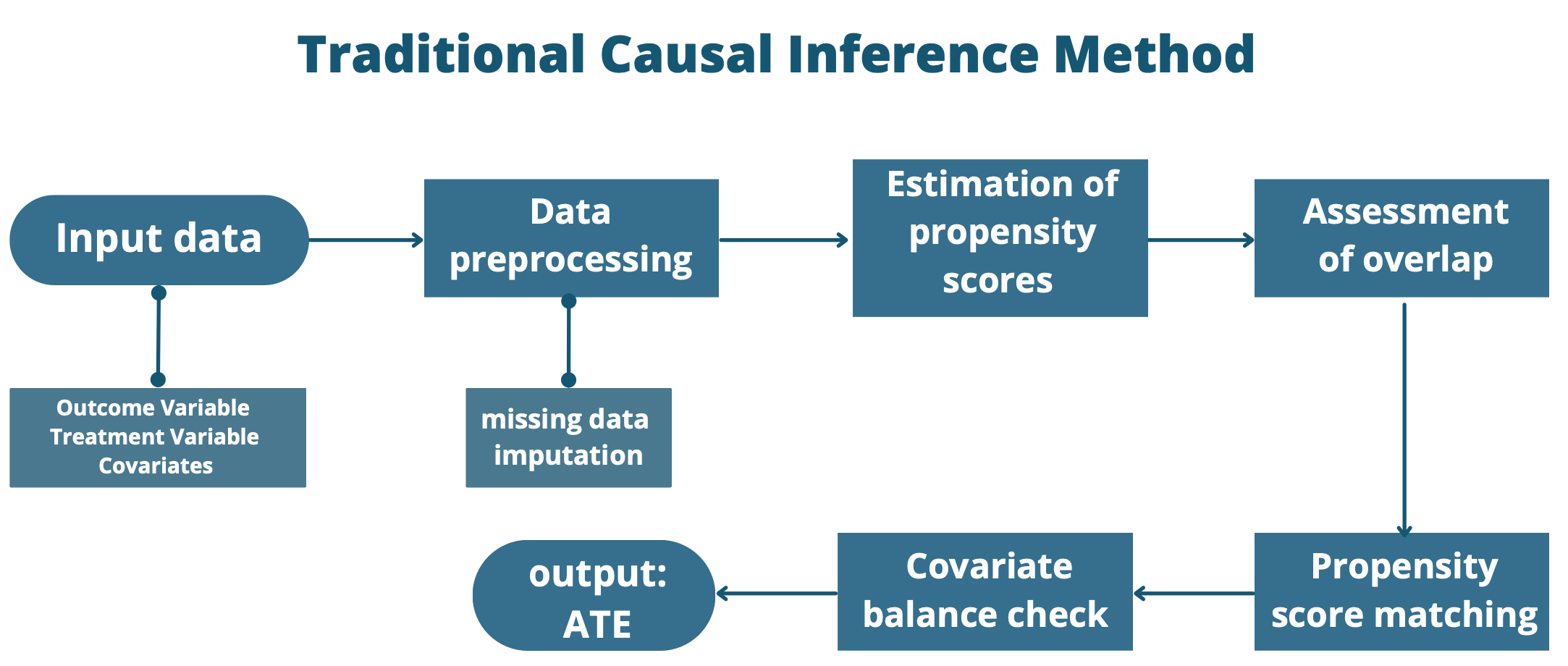
Here is a flowchart explaining the Propensity Score Matching (PSM) commonly used in traditional causal inference methods.

3.2. Causal inference method with machine learning

3.2.1. Ordinary least squares. Ordinary Least Squares (OLS) is sometimes to estimate the linear regression equation and predict \( y \) by \( x \) . Assuming there is a binary treatment variable, \( T \) , where \( T=1 \) for treated units and \( T = 0 \) for untreated units, \( X \) is a matrix of covariates and an outcome variable \( Y \) . The OLS regression model to infer the causal effect of a treatment \( T \) on an outcome \( Y \) is below:

\( Y=α+βT+γX+ϵ \) (13)

There are some basic assumptions in Ordinary Least Squares (OLS). Linearity: The independent and dependent variables have a linear relationship. No endogeneity: The error term and the independent variables are not correlated which can be represented as \( cov(X,ϵ)=0 \) . Homoscedasticity: The error term is distributed with a mean of zero and a constant variance. which can be represented as \( E(ϵ)=0,Var(ϵ)={σ^{2}} \) . No autocorrelation: The error terms are uncorrelated with each other which can be represented as \( cov({ϵ_{i}}{ϵ_{j}})=0 for i≠j \) . No multicollinearity: There was no high correlation between the variables.

OLS method will estimate the coefficients that minimize the sum of squared errors:

\( Q(α,β,γ)=\sum _{i=1}^{n}{[{Y_{i}}-E({Y_{i}})]^{2}}=\underset{α,β,γ}{min}{\sum _{i=1}^{n}{({Y_{i}}-α-β{T_{i}}-γ{X_{i}})^{2}}} \) (14)

Then, solving three equations below simultaneously to get the OLS estimates:

\( \begin{cases} \begin{array}{c} \frac{∂Q}{∂α}=-2\sum _{i=1}^{n}({Y_{i}}-α-β{T_{i}}-γ{X_{i}})=0 \\ \frac{∂Q}{∂β}=-2\sum _{i=1}^{n}{(Y_{i}}-α-β{T_{i}}-γ{X_{i}}){T_{i}}=0 \\ \frac{∂Q}{∂γ}=-2\sum _{i=1}^{n}{(Y_{i}}-α-β{T_{i}}-γ{X_{i}}){X_{i}}=0 \end{array} \end{cases} \) (15)

These three equations can be written in matrix notation:

\( {X^{ \prime }}Xβ={X^{ \prime }}Y \) (16)

So, the ordinary least squares estimation of parameters is:

\( \hat{β}={{(X^{ \prime }}X)^{-1}}{X^{ \prime }}Y \) (17)

\( \hat{β} \) gives a vector of the estimated parameters ( \( \hat{α},\hat{β},\hat{γ} \) ). But OLS provides an unbiased estimate of the ATE only if OLS assumptions are met and conditional independence holds., which suppose \( T \) is randomly assigned binary random variable and \( X \) is independent of \( Y \) . We can estimate \( β \) to know the causal effect and \( \hat{β} \) is the average treatment effect. The sample regression coefficient \( \hat{β} \) based on OLS is a reliable estimator that consistently estimates the causal effect parameter.

3.2.2. Multi-layer perception. Multi-Layer Perception (MLP) is a simple and classical neural network, and it is a supervised learning algorithm. A multi-layer perceptron consists of an input layer, an output layer, and one or more hidden layers. Each neuron node has a nonlinear activation function, except for input nodes. MLP assumes that the relationships between the inputs and the output are not linear. It initializes the weights and biases randomly. Based on the chain rule of differentiation and gradient descent algorithm, MLP assumes that the weights and biases are adjusted by propagating the error backward through the network.

In the first step, this paper inputs the data and initializes the MLP. The input layer consists of a set of neurons \( \lbrace {x_{i}}\rbrace \) which represents the input features. Then training the MLP involving forward propagation, cost computation, and backpropagation. In the hidden layer, each neuron calculates the value of the previous layer through a weighted linear summation. Neurons receive inputs \( X \) and match them with weights \( W \) :

\( {w_{1}}{x_{1}}+{w_{2}}{x_{2}}+⋯{+w_{i}}{x_{i}} \) (18)

the resulting sum is added to the bias \( b \) and passed to the non-linear activation function \( f(∙) \) . Here this paper uses the sigmoidal function as an activation function:

\( f(x)=\frac{1}{1+{e^{-x}}} \) (19)

Each neuron value \( h \) can be calculated using the following formula:

\( {Z_{h}}={W_{h}}{h_{prev}}+{b_{h}} \) (20)

\( h=f({Z_{h}}) \) (21)

where \( h \) represents the output of the hidden layer, \( {h_{prev}} \) represents the output of the previous layer, \( {W_{h}} \) represents the weight matrix of the hidden layer, and \( {b_{h}} \) represents the bias vector of the hidden layer. The output layer takes the last hidden layer's value and converts it to the output.

In this process, this paper calculates the loss function to measure the error between the model's predictions and the real data. The loss function for an MLP is usually the Mean Squared Error (MSE), which can be computed as:

\( L=\frac{1}{n}\sum _{i=1}^{n}{(y-\hat{y})^{2}} \) (22)

where \( n \) is the number of samples, \( y \) is the target output, \( \hat{y} \) is the predicted output.

To minimize the loss function, this paper uses error Back-Propagation algorithm to adjust the parameters and we commonly use the gradient descent algorithm. This paper calculates the error gradient for each neuron by backpropagation and update the weights and biases between neurons using gradient descent. This can be represented by the following equations:

\( \frac{∂L}{∂{W_{h}}}=\frac{∂L}{∂f({Z_{h}})}∙\frac{∂f({Z_{h}})}{∂{Z_{h}}}∙\frac{∂{Z_{h}}}{∂{W_{h}}} \) (23)

\( \frac{∂L}{∂{b_{h}}}=\frac{∂L}{∂f({Z_{h}})}∙\frac{∂f({Z_{h}})}{∂{Z_{h}}}∙\frac{∂{Z_{h}}}{∂{b_{h}}} \) (24)

\( {W_{h}}={W_{h}}-η\frac{∂L}{∂{W_{h}}} \) (25)

\( {b_{h}}={b_{h}}-η\frac{∂L}{∂{b_{h}}} \) (26)

where \( η \) is the learning rate.

Then, this paper can make predictions after the MLP is trained. The prediction \( \hat{y} \) can be computed by applying the forward propagation step to the test data:

\( \hat{y}=f({W_{h}}{h_{prev}}+{b_{h}}) \) (27)

Finally, calculating the difference in predicted outcomes between the treated and untreated units and the ATE is:

\( ATE=E({\hat{y}_{treated}})-E({\hat{y}_{untreated}}) \) (28)

3.2.3. Targeted maximum likelihood estimation. Targeted Maximum Likelihood Estimation (TMLE) is a doubly robust maximum likelihood-based estimator. The TMLE approach is useful in achieving the optimal balance between the bias and variance tradeoff for the target parameter, and we will get more valid inferences. Let \( T \) denote the binary treatment variable, \( W \) denote the vector of potential confounders of treatment and outcome, and \( Y \) denote the continuous outcome. There are several assumptions made in the Rubin causal framework. The SUTVA assumes that the exposure status of one individual does not have an impact on the potential outcomes of another individual. Another causal assumption includes no unmeasured confounders and positivity. They are formalized as \( ({Y_{1}},{Y_{0}})⊥T|W \) and \( 0 \lt P(T=1|W) \lt 1 \) .

TMLE can estimate initial outcomes \( Q(T,W) \) , and probability of treatment \( g(W) \) and produce an updated estimate \( {Q^{*}}(T,W) \) . Steps to implement TMLE to estimate ATE are as follows.

The first step is to use confounders and treatment status as predictors to estimate the expected outcome for all observations. This article generates the initial estimate:

\( Q(T,W)=E[Y|T,W] \) (29)

Then this article uses the confounders as predictors to estimate all observations' probability of receiving the treatment which is often called the propensity score:

\( g(W)=P(T=1|W) \) (30)

With propensity scores, we can compute the prediction of two probabilities: inverse probability of receiving treatment \( \frac{1}{\hat{P}(T=1|W)} \) and negative inverse probability of not receiving treatment \( -\frac{1}{\hat{P}(T=0|W)} \) . Then this article can get the clever covariate:

\( H[T,W]=\frac{I(T=1)}{\hat{P}(T=1|W)}-\frac{I(T=0)}{\hat{P}(T=0|W)} \) (31)

To make our estimate of the ATE is asymptotically unbiased, this article updates the initial estimate of \( E[Y|T,W] \) . This paper will solve an equation to figure out how much to update:

\( logit(E[Y|T,W])=logit(\hat{E}[Y|T,W])+ϵH(T,W) \) (32)

To solve this equation, this article fits a logistic regression with the clever covariate \( H[T,W] \) , initial outcome estimates \( logit(\hat{E}[Y|T,W]) \) and the outcome \( Y \) . The \( expit \) can be used to get the inverse of \( logit \) function so the initially expected outcome estimates will be updated:

\( {\hat{E}^{*}}[Y|T,W]=expit(logit(\hat{E}[Y|T,W])+\hat{ϵ}H(T,W)) \) (33)

Calculate the ATE according to the updated expected outcomes estimates as follows:

\( \hat{{ATE_{TMLE}}}=\frac{1}{N}\sum _{i=1}^{N}{\hat{E}^{*}}[Y|T=1,W]-{\hat{E}^{*}}[Y|T=0,W] \) (34)

3.2.4. Bayesian additive regression trees. The Bayesian Additive Regression Trees (BART) can be described as a model that combines a multitude of decision trees and a regularization prior. The building block of BART is regression trees. Regression trees predict the \( y \) using trees \( {T_{l}}, 1≤l≤L \) , which means a series of if-else conditions with each partition \( {A_{b}} \) , based on the value of \( x \) , sets a constant value \( {m_{lb}} \) to \( y \) .

There is also a set of parameter constraints or priors that regularize the split likelihood. So, this article can define a constant function combined with the partition, the parameters, and the priors:

\( {g_{l}}(x)={m_{lb}} if x∈{A_{b}} \) (35)

Then a resemble of individuals are amalgamated into a singular regression forest:

\( Y=\sum _{l=1}^{L}{g_{l}}(x)+ϵ \) (36)

The BART model can be represented as:

\( Y=g(z,x;{T_{1}},{M_{1}})+g(z,x;{T_{2}},{M_{2}})+…+g(z,x;{T_{m}},{M_{m}})+ϵ=f(z,x) \) (37)

which defines \( g(z,x;T,M) \) as the value obtained by following observation \( (z,x) \) down a tree and returning mean for the terminal node in which it lands, \( M=\lbrace {μ_{1}},{μ_{2}},⋯{μ_{b}}\rbrace \) as the vector of means in the b terminal nodes of the tree.

To prevent overfitting and limit the range of reasonable errors, BART regularization is essential. Regularization prior prefers fewer nodes and the probability associated with a node at depth \( h \) undergoing a split are:

\( η{(1+h)^{-β}} with default η=0.95 and β=2 \) (38)

It also shrinks the effect of predictor toward zero:

\( {m_{lb}}~N(0,σ_{m}^{2}), {σ_{m}}=\frac{{σ_{0}}}{\sqrt[]{L}} \) (39)

The fundamental procedures for estimating the causal impact utilizing BART are outlined below:

The first thing is to input variables \( Y, X,Z \) to the MCMC random forest with regression parameter specification. The posterior can be computed by using MCMC after a prior putting on the parameters. MCMC is Markov chain Monte Carlo, which seeks out a good \( f \) by using a stochastic search for each tree. At each iteration, each \( ({T_{j}},{M_{j}}) \) and \( σ \) are redrawn and the BART function will be updated by parameters. Each iteration generates a new draw of \( f \) and prediction on \( Y \) . According to MCMC random forest, this article can get a function:

\( [Y|(X,Z)]=f(x,z) \) (40)

and do some prediction with calculating \( f(x,z=1) \) and \( f(x,z=0) \) . The posterior distribution of \( f(X,Z) \) can be known. So, this article straightforward gets an estimation of the causal effect from posterior distribution:

\( τ(x)=f(x,z=1)-f(x,z=0) \) (41)

Considering the conditions on the \( X \) values, this article calculates the conditional average treatment effect (CATE):

\( \frac{1}{n}\sum _{i=1}^{n}f({x_{i}},z=1)-f({x_{i}},z=0) \) (42)

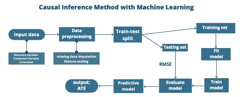
The following flowchart represents the basic machine learning steps in causal inference.

4. Results

4.1. Data description

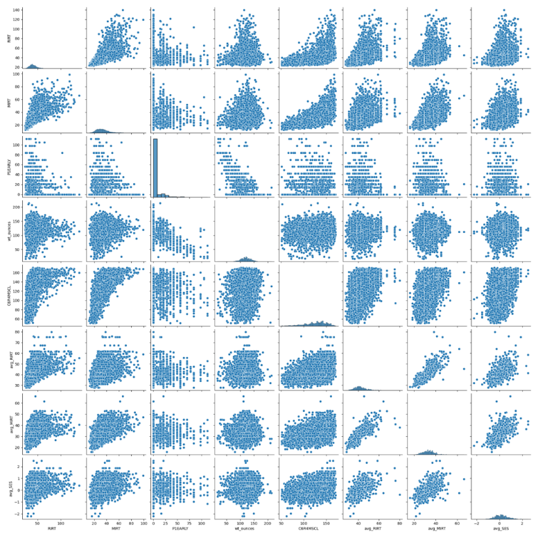
This paper uses data from the 1998-1999 Early Childhood Longitudinal Study of Kindergarten Classes (ECLS-K) to estimate the average treatment effect (ATE) of receiving special education services. After deleting cases with missing variate information, there are 36 variables with a sample size of 7362. The treatment variable is whether students receive special education services or not, 429 students in our dataset are enrolled in special education services. The outcome variable is the fifth-grade math score, ranging from 50.9 to 170.7. The other variables include demographic, academic, school composition, family context, health, and parent rating of the child. In our dataset, there are 3657 male and 3705 female cases. 5759 students were in the public school and 96.7% of students were first-time kindergarteners. In their family context, 6193 students got nonparental Pre-K childcare and 1265 students were from one-parent families. Here this article uses the Python package seaborn to create a plot that can describe variables’ distributions. When dealing with a large number of variables, it is important to visualize their relationships through a heatmap to identify strongly correlated variables. First, this article creates a heatmap and then generates a correlation graph for the chosen variables. The darker shades in the heatmap indicate a stronger correlation between the variables. In the correlation graph, the diagonal plots show the distribution of each variable, and the off-diagonal plots show the relationship between two different variables.

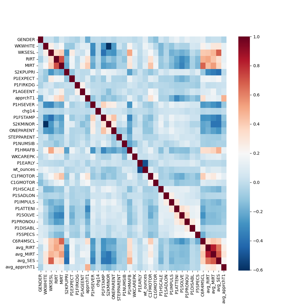
According to the figures, this article finds a positive correlation between kindergarten reading scores and kindergarten math scores, reading IRT and math IRT, math IRT, and SES. This article also finds a negative correlation between birth weight and number of days premature. Considering fifth-grade math scores, it is positively correlated with kindergarten reading scores and kindergarten math scores, negatively correlated with problem-solving.

4.2. Average treatment effect

This article uses five methods to calculate average treatment effects (ATE). In the traditional method of causal inference, this article uses propensity score matching (PSM) by following the steps below: estimation of propensity scores with logistic regression, performing matching, assessment of overlap, assessment of covariate balance, and calculating ATE. In the steps of machine learning, this article did a train-test split first with 0.25 test size. After selecting the model, this article trained the model with default parameters. To get the predictions for the counterfactual outcome, this article assigns all treatments to 1 and 0 respectively. After predicting two counterfactual outcomes, this article calculates the ATE through them.

The table displays results for ATE with different methods. In general, the results are all less than 0, which means the students who took special education services didn’t perform better than other students. Participating in special education services is not the reason for higher math grades. This may be due to the differences in the endowments of these students or their academic abilities. In the traditional causal inference method, the result of ATE is -3.175. In the machine learning method, MLP’s predicted performance is the best with its minimum variance, and the result is -1.051. BART also performed well, and its result is close to the MLP. However, OLS and TMLE didn’t perform as well as BART and MLP. Machine learning methods will get smaller variance than traditional methods.

Table 1. Results of different methods.

4.3. Factor analysis

In further studies, this article hopes to identify the factors that affect students' math scores or the reasons for their improvement. Given the number of variables studied, this article uses principal component analysis (PCA) to reduce dimension for further study. First, analyze whether the research data is suitable for PCA. As can be seen from the table above, KMO is 0.799, greater than 0.6, which meets the prerequisite requirements of PCA. The dataset successfully met the criteria of Bartlett’s Test of Sphericity \( (p \lt 0.05) \) , thereby affirming its appropriateness for PCA.

Table 2. KMO and Bartlett's test of Sphericity.

The table and scree plot reveal that twelve principal components have been extracted, each with eigenvalues exceeding one. The variance of the main components of 12 explained rates were 16.873%, 6.913%, 5.036%, 4.463%, 4.175%, 3.678%, 3.510%, 3.335%, 3.161%, 3.134%, 3.034%, 3.003%, and the cumulative variance explained at a rate of 60.315%.

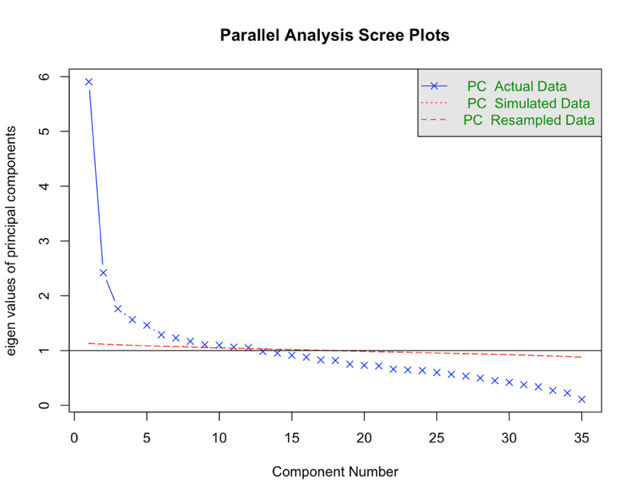
Table 3. Eigenvalue and variance contribution.

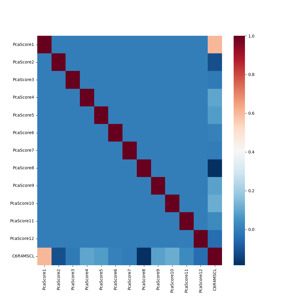
This article analyzes the correlation between 12 principal components and fifth-grade math scores and finds that the first principal component has a strong positive correlation with the score. By observing the load coefficient, it can be explained as students’ academic ability and their education context. A student who has perfect academic ability and gets a high-quality education may get higher math scores. The second and the eighth principal components negatively correlate with the score. They can be explained as the parent rating of the child. The reason for the negative correlation probably is too much parental discipline is counterproductive. In the process of further studying the variables that have a causal relationship with math grades, this article studies the academic ability, educational background, and parent rating of the child.

5. Conclusion

In this article, our study tried to explore the causal relationship between access to special education and fifth-grade math scores. Whether students can improve their math scores after receiving special education is our concern. In estimating causal effects, this article utilized traditional causal inference methods as well as machine learning techniques. It is crucial to pay attention to the promising area of development that lies at the intersection of causal inference and machine learning. Machine learning can improve the accuracy and efficiency of estimating causal effects as more data is processed. It is possible to determine the effectiveness of a machine learning model by examining its prediction variance. A model with a smaller prediction variance is considered good. Regarding our main concern, the average treatment effect of negative values indicates that there is no causal effect on special education and math scores. Participating in special education does not necessarily result in higher math grades. It could be attributed to variations in students' endowments, abilities, or limitations in the data set under investigation. Given the complexity of our data, this paper performed factor analysis to facilitate further investigation. After conducting principal component analysis on variables, this paper found 12 principal components and discovered that students with exceptional academic abilities and who receive a high-quality education tend to perform better on math scores as well. However, excessive parental input may have a negative impact on the child's performance. The potential causal relationships between these factors and students' math performance could be further explored through in-depth causal inference analyses in future studies.

References

[1]. Holland, P. W. (1986). "Statistics and Causal Inference." Journal of the American Statistical Association, 81(396), 945-960.
[2]. Rubin, D. B. (2005). "Causal Inference." Journal of Causal Inference, 3(2), 105-133.
[3]. McConnell, K. J., & Lindner, S. (2018). "Estimating Treatment Effects with Machine Learning." Health Services Research, 53(2), 802-823.
[4]. Hill, J. L. (2011). "Bayesian Additive Regression Trees: A Review and Look Forward." Statistical Science, 26(1), 102-115.
[5]. Keller, B., & Tipton, E. (2016). "Propensity Score Analysis in R: A Software Review." Journal of Educational and Behavioral Statistics, 41(2), 205-233.
[6]. Hume, D. (1748). An Enquiry Concerning Human Understanding, Section VII.
[7]. Lewis, D. (1973). "Causation." Journal of Philosophy, 70, 556-567.
[8]. Neyman, J. (1923). "On the Application of Probability Theory to Agricultural Experiments. Essay on Principles. Section 9." Statistical Science, 5(4), 465–472.
[9]. Fisher, R. A. (1935). The Design of Experiments. Oliver and Boyd.
[10]. Rubin, D. B. (1974). "Estimating Causal Effects of Treatments in Randomized and Nonrandomized Studies." Journal of Educational Psychology, 66(5), 688–701.
[11]. Liu, Y., Li, X., & Zhang, J. (2019). "Propensity Score Analysis: A Review and a Case Study." Journal of Data Science, 17(2), 305-321.
[12]. Keller, B., & Tipton, E. (2016). "Propensity Score Analysis in R: A Software Review." Journal of Educational and Behavioral Statistics, 41(3), 326-348.
[13]. Pearl, J. (2009). "Causal Inference in Statistics: An Overview." Statistics Surveys, 3, 96-146.
[14]. Pearl, J. (1995). "Causal Diagrams for Empirical Research." Biometrika, 82, 669-688.
[15]. Pearl, J. (2000). Causality: Models, Reasoning, and Inference. Cambridge University Press, pp. 69-146, 205-278.
[16]. Van der Laan, M. J., & Rose, S. (2018). Targeted Learning: Causal Inference for Observational and Experimental Data. Springer Science & Business Media.
[17]. Schuler, M. S., & Rose, S. (2017). "Targeted Maximum Likelihood Estimation for Causal Inference in Observational Studies." American Journal of Epidemiology, 185(1), 65-73.
[18]. Gruber, Susan. (2019). tmle: An R Package for Targeted Maximum Likelihood Estimation. R package version 1.5.0.
[19]. Chipman, H. A., George, E. I., & McCulloch, R. E. (2010). "BART: Bayesian Additive Regression Trees." The Annals of Applied Statistics, 4(1), 266-298.
[20]. McCulloch, R., Chipman, H., & George, E. (2019). bart: Bayesian Additive Regression Trees. R package version 2.9.
[21]. Chipman, H. A., George, E. I., & McCulloch, R. E. (2010). "BART: Bayesian Additive Regression Trees." The Annals of Applied Statistics, 4(1), 266-298.
[22]. Hahn, P. R., Murray, J. S., & Carvalho, C. M. (2020). "Bayesian Regression Tree Models for Causal Inference: Regularization, Confounding, and Heterogeneous Effects." Bayesian Analysis, 15(3), 965-992.
[23]. Chernozhukov, V., Chetverikov, D., Demirer, M., Duflo, E., Hansen, C., Newey, W., & Robins, J. (2019). "Double Machine Learning for Heterogeneous Treatment Effects." arXiv preprint arXiv:1902.07409.
[24]. Hill, J. L. (2011). "Bayesian Nonparametric Modeling for Causal Inference." Journal of Computational and Graphical Statistics, 20(1), 217-240.
[25]. McConnell, K. J., & Lindner, S. (2020). "Estimating Treatment Effects with Machine Learning." Health Services Research, 55(1), 5-22.
[26]. Peters, J., Janzing, D., & Schölkopf, B. (2017). Elements of Causal Inference: Foundations and Learning Algorithms. MIT Press.
[27]. Pearl, J. (2000). Causality. Cambridge University Press.
Cite this article
Li,J. (2024). Machine learning for causal inference: An application to ECLS-K data. Applied and Computational Engineering,76,33-47.
Data availability
The datasets used and/or analyzed during the current study will be available from the authors upon reasonable request.
Disclaimer/Publisher's Note
The statements, opinions and data contained in all publications are solely those of the individual author(s) and contributor(s) and not of EWA Publishing and/or the editor(s). EWA Publishing and/or the editor(s) disclaim responsibility for any injury to people or property resulting from any ideas, methods, instructions or products referred to in the content.
About volume
Volume title: Proceedings of the 2nd International Conference on Software Engineering and Machine Learning
© 2024 by the author(s). Licensee EWA Publishing, Oxford, UK. This article is an open access article distributed under the terms and
conditions of the Creative Commons Attribution (CC BY) license. Authors who
publish this series agree to the following terms:
1. Authors retain copyright and grant the series right of first publication with the work simultaneously licensed under a Creative Commons
Attribution License that allows others to share the work with an acknowledgment of the work's authorship and initial publication in this
series.
2. Authors are able to enter into separate, additional contractual arrangements for the non-exclusive distribution of the series's published
version of the work (e.g., post it to an institutional repository or publish it in a book), with an acknowledgment of its initial
publication in this series.
3. Authors are permitted and encouraged to post their work online (e.g., in institutional repositories or on their website) prior to and
during the submission process, as it can lead to productive exchanges, as well as earlier and greater citation of published work (See
Open access policy for details).