1. Introduction

Diabetes is a disease of the endocrine system caused by hyperglycemia, and the number of people with diabetes worldwide is expected to reach 1.31 billion by 2050. Diabetes can cause the tissue cells in the human body to be insufficiently supplied with nutrients for a long period of time, thus leading to various complications [1]. Through the early diagnosis of diabetes, asymptomatic patients and patients with impaired glucose tolerance can be detected in time, and early detection and early treatment can delay and reduce the occurrence of complications [2]. Diabetes diagnosis has age, gender, height, weight, blood pressure, blood lipids and other indicators, but the traditional risk assessment system for diabetes has a large number of indicators, and there is no relative importance between the indicators, so it is difficult to diagnose diabetes through the traditional methods and the accuracy is not high, so a new diabetes diagnosis was urgently needed.

Machine learning models have certain advantages in the medical field. For example, initial diagnosis of diseases can be achieved through decision tree and random forest models. Deep learning is a subfield of machine learning that uses neural network models to learn nonlinear relationships. Deep learning models have greater representational capabilities than traditional machine learning models. In this study, deep neural network based on features such as Body Mass Index (BMI), weight, and blood pressure was used to achieve the diagnosis of diabetes.

2. Method

2.1. Dataset and data preprocessing

2.1.1. Dataset

This section focuses on the datasets used in the study. The two datasets used in this study are from the Kaggle machine learning database, which document information related to diabetic patients from the National Institute of Diabetes and Digestive and Kidney Diseases in the United States of America and from the Frankfurt Hospital in Germany, respectively [3], and contain a total of 2,768 samples.

2.1.2. Data preprocessing

Since the dataset used is the original dataset recorded by the hospital and the institute, the dataset suffers from problems such as incomplete data and incorrect data recording. Therefore, it is necessary to preprocess the dataset in this study, and the missing values present in the dataset were processed and the missing data are shown in Table 1. For all five attribute columns, the missing value filling was accomplished using the plurality method.

Table 1. Missing values for each column of the dataset

2.1.3. Data balancing

Through statistical analysis of the data, there was a problem of balanced data distribution for both labels. As shown in Figure 1(a) the diabetic and do not suffer from diabetes is close to 2:1.

The data imbalance makes the experimental model much less effective. In order to solve this problem, this study adopted the Synthetic Minority Over-sampling Technique (SMOTE) method for data resampling, which is used to effectively deal with the unbalanced learning problem [4]. The specific method is as follows.

\( c= a + λ ( b - a )\ \ \ (1) \)

where c is a synthetic sample, a is a positive class sample, a random number between 0 and 1, the weight of the difference vector, and b is the nearest-neighbor sample of an obtained by Euclidean distance. After the experimental processing, as in Figure 1(b), the number of samples labeled 0 and labeled 1 were almost balanced.

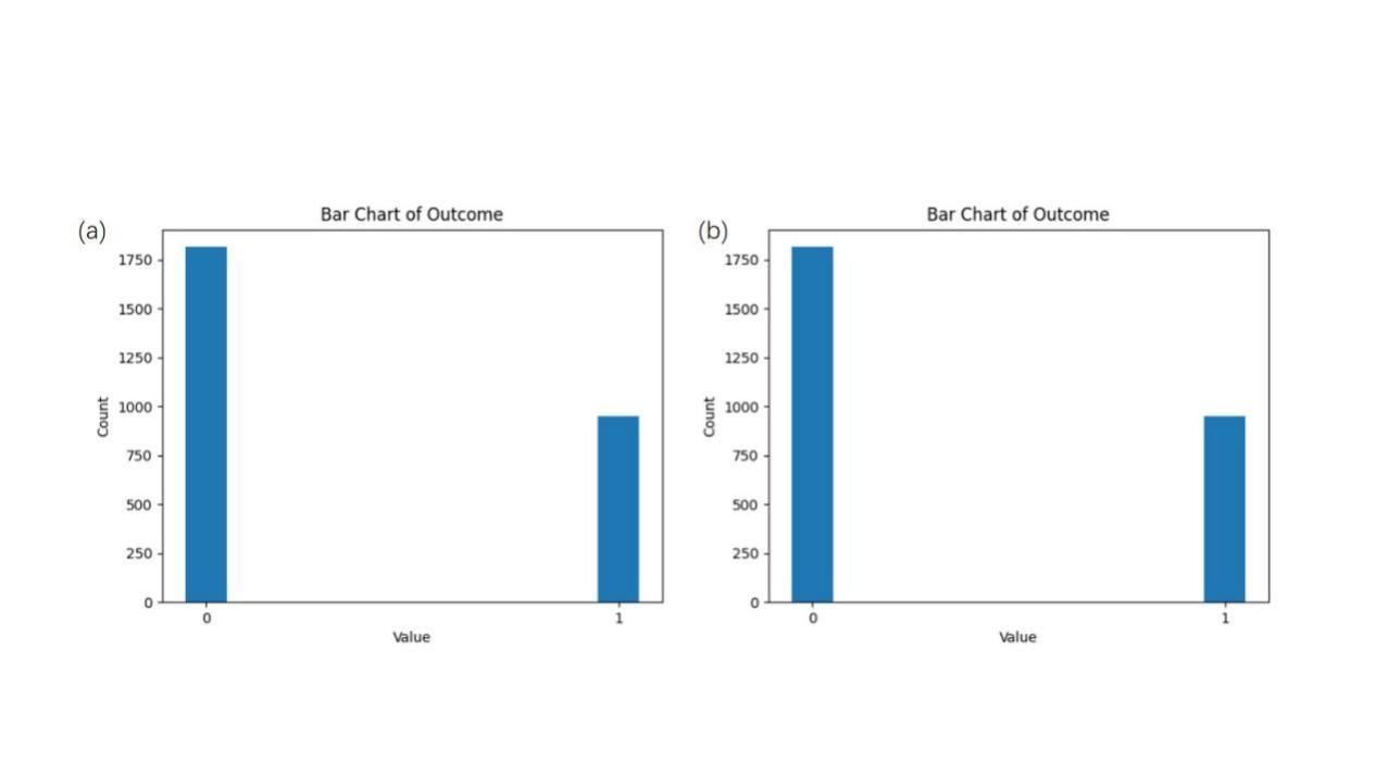
Figure 1. Labeling statistics. (a) The distribution of data before resampling. (b) The distribution of data after resampling.

2.1.4. Data feature selecting

In this study, deep learning algorithms were applied to the research. Although deep learning algorithms were capable of filtering features, considering that some of the information in the dataset may not be relevant to the purpose of the research, some meaningless information may even affect the realization of the experimental purpose. Therefore, it is necessary to filter and select features to ensure that the features used can better serve the research purpose.

The Spearman correlation coefficient [5] of each feature with the label ‘Outcome’ was calculated as follows.

\( Ρ=\frac{\sum _{i} ({x_{i}}-\bar{x})({y_{i}}-\bar{y})}{\sqrt[]{\sum _{i} ({x_{i}}-\bar{x}{)^{2}}\sum _{i} ({y_{i}}-\bar{y}{)^{2}}}}\ \ \ (2) \)

where x and y are the two features of the computation. Choosing 0.1 as the threshold for feature selecting, the heat map obtained is shown in Figure 2

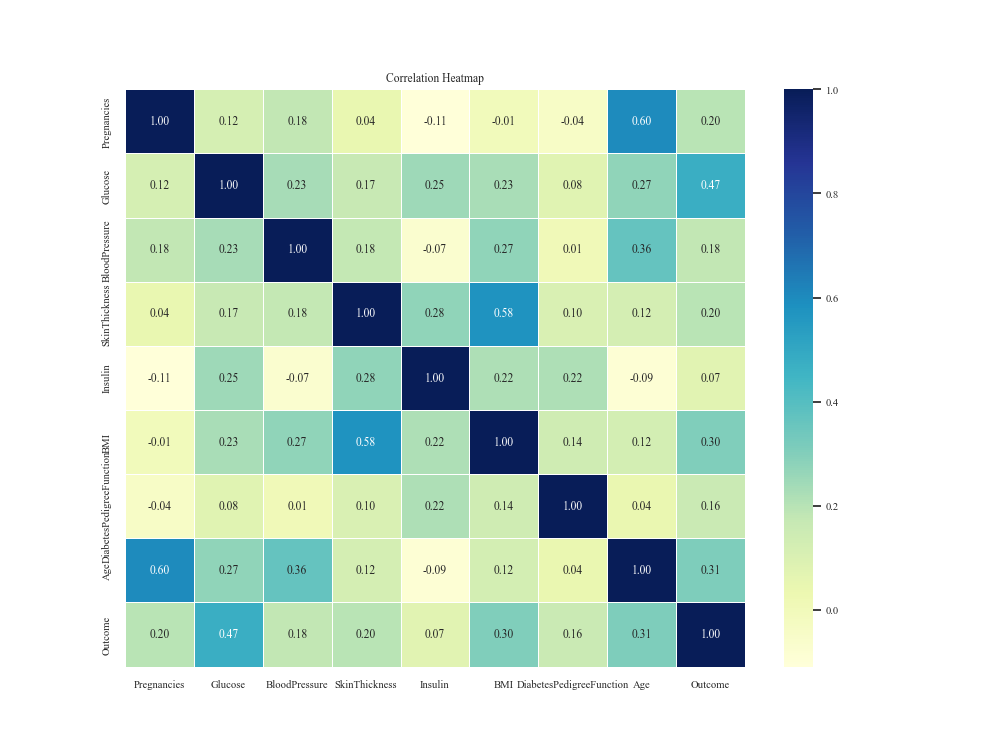
Figure 2. Features heat map.

The results showed that the three features with the highest correlation coefficients were Glucose, DiabetesPedigreeFunction, and BMI, while there were seven features with Spearman's correlation coefficients greater than 0.1, and one Insulin (serum insulin two hours after a meal) less than 0.1, so the remaining seven important features were selected.

2.1.5. Data distribution analysis

The data distribution analysis was carried out on the seven features of the dataset. Figure 3 shows the distribution of the dataset. There is a strong nonlinear correlation between the features Glucose, observations, Age and labels, while DNN has a strong nonlinear function fitting ability, so it performed well in this study with outstanding indicators.

.

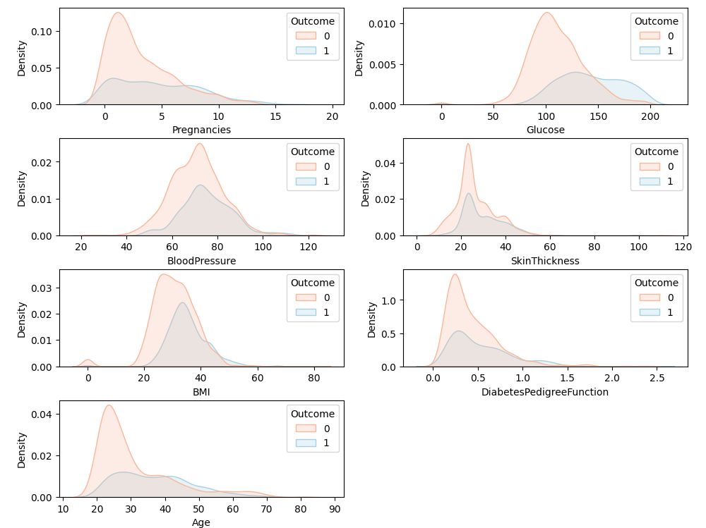
Figure 3. Data distribution analysis

2.1.6. Data normalization

In the data set of this study, there were large numerical differences between different features, and the influence of dimension needed to be eliminated. Therefore, Min-Max normalization was used to map the result value to the range [0-1], as follows:

\( {x_{new}}=\frac{x-{x_{min}}}{{x_{max}}-{x_{min}}}\ \ \ (3) \)

where \( {x_{new}} \) is the value of the feature after normalization, \( { x_{max}}{x_{min}} \) is the maximum and minimum value of the feature in the data set, respectively.

3. Models

3.1. Deep neural network

Compared to traditional neural networks, DNN has a deeper network structure that captures high-level abstractions in the data and obtains better nonlinear fitting ability through activation functions [6]. Among the DNN-based diabetes diagnosis, a 7-layer deep neural network was built, as shown in Figure 4.

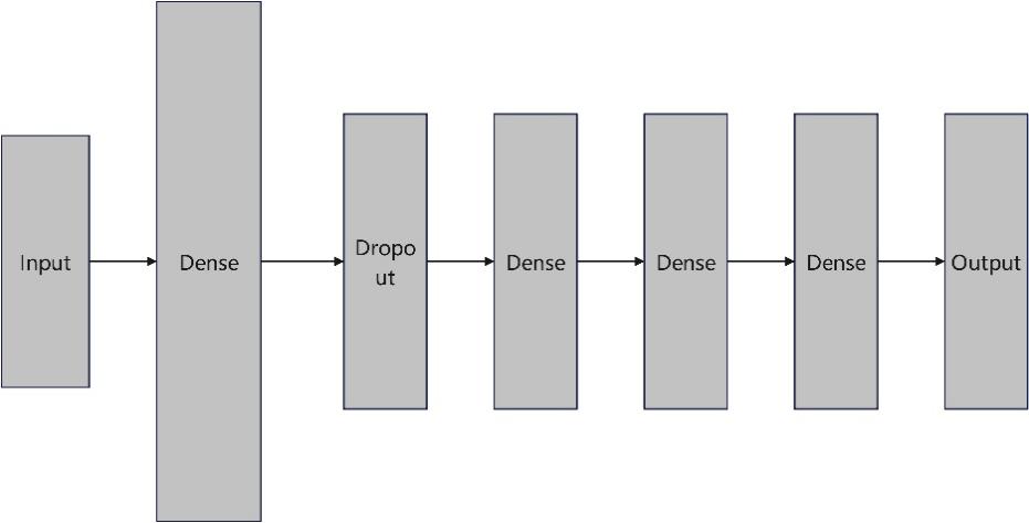
Figure 4. DNN structure.

First, an input layer of 7 neurons was designed, as the dataset retained 7 features after feature filtering. Then a fully connected layer of 128 neurons is connected to perform preliminary processing and feature extraction on the input data. By using the Relu function as an activation function, the nonlinear fitting ability of the model was improved. Further, a Dropout layer is set to deactivate 10% of the random neurons to prevent overfitting of the neural network and to improve robustness. The fully connected layer method with Relu function is as follows.

\( y=w*x+b\ \ \ (4) \)

\( f(x)=max{(0,x)}\ \ \ (5) \)

In order to learn more nonlinear relationships between features and labels, two fully connected layers with 64 and 32 neurons were then set up to extract higher level abstract features, again using the Relu function as the activation function to learn nonlinear relationships.

Finally, a fully connected layer with only one neuron was set up and a Sigmoid function was set to convert the output of the network to a probability value between 0 and 1 for classification judgment. In situations where the output value exceeds 0.5, the model indicates that the input data falls into the positive category; in situations where the output value is below 0.5, the model indicates that the input data falls into the negative category. The Sigmoid function is as follows.

\( f(x)=\frac{1}{1+{e^{-x}}}\ \ \ (6) \)

3.2. Machine learning models

3.2.1. Logistic regression

Logistic regression (LR) belongs to linear classifiers, through the Logistic function, the data features are mapped to the probability value of a sample belonging to a positive example in the interval 0 to 1, and the classification to which the data belongs is derived by comparing it with 0.5 [7]. The principle of calculation is as follows.

\( f(x)=\frac{1}{1-{e^{-z}}}\ \ \ (7) \)

\( z={w^{T}}+{w_{0}}\ \ \ (8) \)

3.2.2. Decision trees

The predictive model of a decision tree (DT) shows the mapping relationship between object values and characteristics. Every leaf node in the tree corresponds to the value of the object represented by the path traveled from the root node to that leaf node, each forked path in the tree represents a potential attribute value, and each node in the tree represents a specific item [8]

3.2.3. Gradient Boosting

Gradient Boosting (GBDT), a predictive model based on statistics and machine learning, is widely used in a variety of data science fields, including but not limited to time series analysis, classification, regression, ranking, etc. GBDT is an integrated learning method that allows the construction of a strong-learning predictive model by combining the prediction results of multiple weak-learning predictive models. The core idea of GBDT is to select an optimal basis function in each iteration so that the weighted sum of the basis function and the residuals is minimized. In the training process, GBDT uses a loss function called "boosting" and a weakly learned model called "base learner" for training. In this way, GBDT can gradually improve the prediction results and eventually reach a relatively stable model [9].

3.2.4. Adaptive Boosting

Adaptive Boosting (AdaBoost) combines several weak classifiers to create a strong classifier. In the AdaBoost algorithm, a new classifier is trained in each iteration and the sample weights are adjusted according to the performance of the previous round of classifiers, so that the samples that have been misclassified in the training data are given more attention in the next round. It forces the classifiers that come after to focus more on the samples that are prone to incorrect classification. AdaBoost's fundamental concept is to create a strong classifier by merging several weak classifiers, which increases classification accuracy overall. In each round of training, AdaBoost will adjust the weights of the samples according to the performance of the previous round of classifiers, so that the previously misclassified samples will be more likely to be correctly classified in the next round [10].

3.3. Neural network training

The processed dataset in this study was split into training and testing sets at an 8:2 ratio, which was utilized to train the DNN using the model's evaluation. The DNN model was trained for 500 epochs, and the model was built and trained based on the Keras platform of Tensorflow, using the Adam optimizer to reduce the loss function binary_crossentropy. The learning rate was set to 0.001, α was set to 0.9, β was set to 0.999, and at the end of each round of training, a new loss function was calculated. The code was performed on an NVIDIA 3070 GPU.

3.4. Evaluation metrics

The problem of this study is a dichotomous classification problem to diagnose the presence of diabetes. Therefore Accuracy (Acc) is one of the most important indicators and its value is equal to the percentage of correctly categorized samples out of the total samples. Also, in order to minimize the occurrence of underdiagnosis, Recall (Rec), which is an important indicator, is the probability that a patient with diabetes is diagnosed as not having diabetes. In this study, the F1 score is able to consider both the accuracy and coverage of the model, and is able to find a balance between accuracy and recall, which is also an important indicator. Reducing false positives is also important, so Precision (Prec) was chosen as an important metric to indicate the proportion of samples predicted by the model to be diabetic that are diabetic. In addition, area under the curve (AUC) is often used to measure the generalization ability of the model and is calculated from the area under the receiver operating characteristic curve (ROC) curve.

4. Results

4.1. Neural network training results

Figure 5 illustrated the training results of the neural network. It can be seen that the loss of the model decreased rapidly in epochs 0 to 200 and gradually levels off in epochs 200 to 500, while the accuracy of the model on the test set increased rapidly in epochs 0-250 and levels off in epochs 250-500.

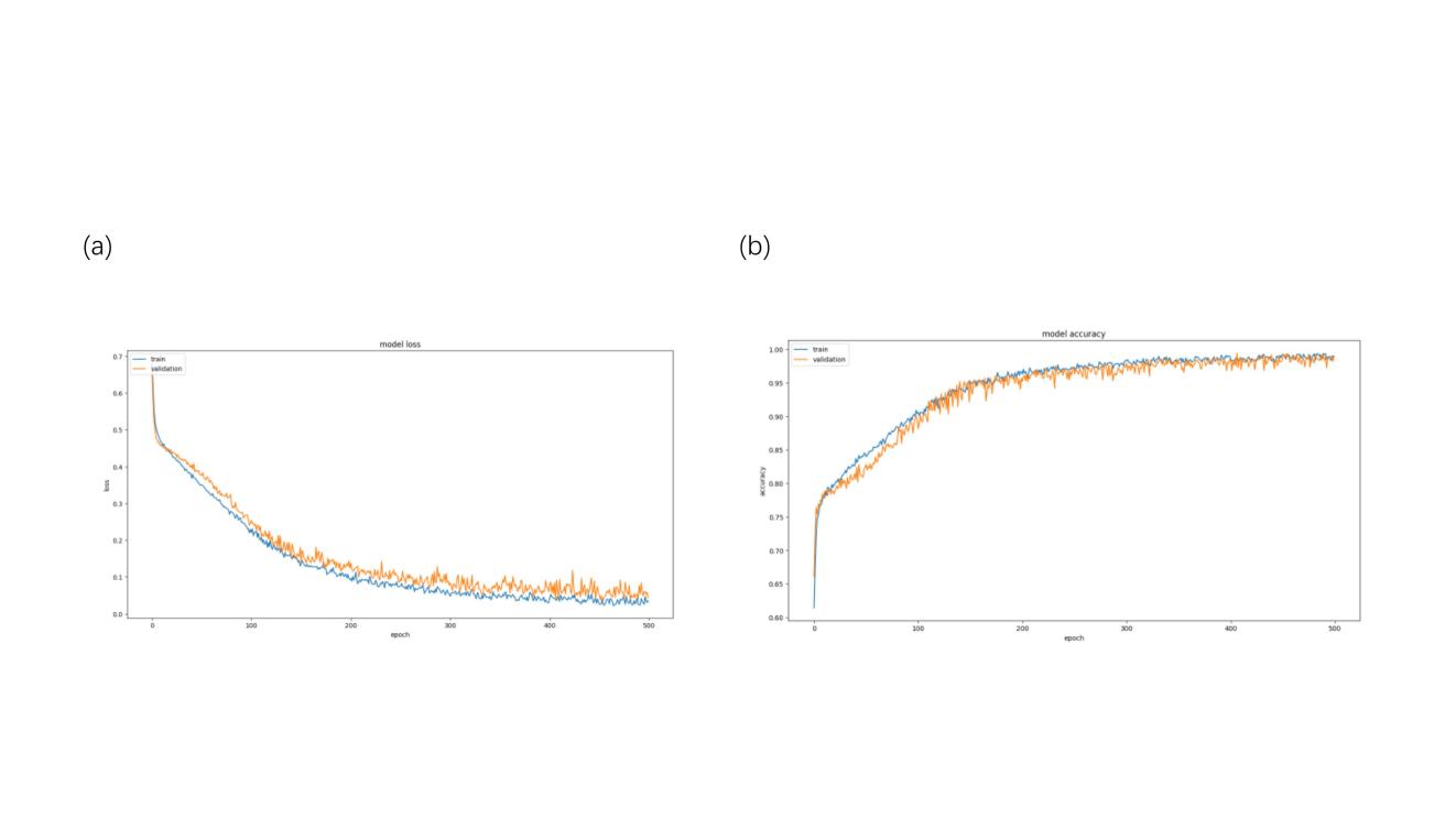
Figure 5. Network training visualization. (a) Loss curve. (b) Accuracy curve.

4.2. Deep neural network prediction results

In this study, the processed dataset was divided into training and test sets in the ratio of 8:2, and the metrics of DNN on the test set are shown in Figure 6. From the results, it can be seen that DNN achieved 99.5% accuracy Acc on the test set, which ensures the accuracy of diagnosis, while AUC achieves 99.8%, which indicates that DNN possesses strong generalization ability, Precision achieves 1 and 99.6% on the two types of samples, while Recall achieves 99.1% vs. 1 on the two types of samples, which ensures that missed diagnosis with false alarms occurrences were low.

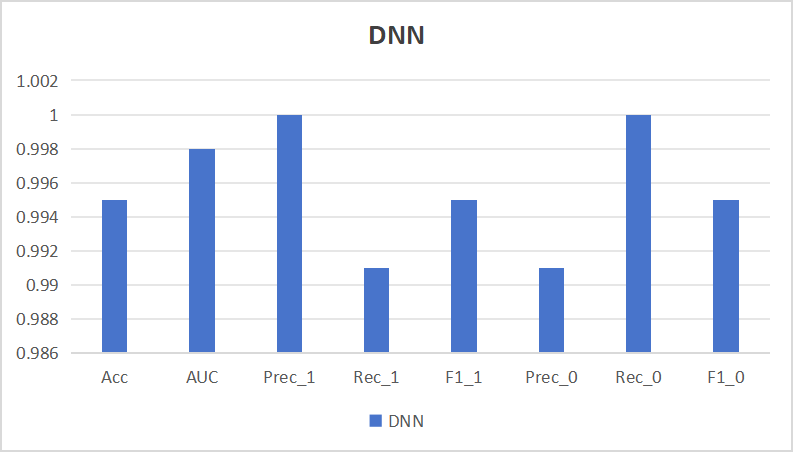
Figure 6. The evaluation metrics of DNN.

4.3. Model comparison

In this study, LR, DT, GBDT, AdaBoost and XGBoost were selected to compare with DNN, and the results are shown in Table 2 with Figure 7. From the chart, DNN outperforms the remaining five machine learning models in the indicators of Acc, AUC, Prec, Rec, and F1. The diagnostic accuracy was the highest, with Acc reaching 99.5%, and the least number of omissions and false alarms occurring, and the highest indicator of AUC also reflected the strong robustness of DNN.

Table 2. Evaluation metrics of models

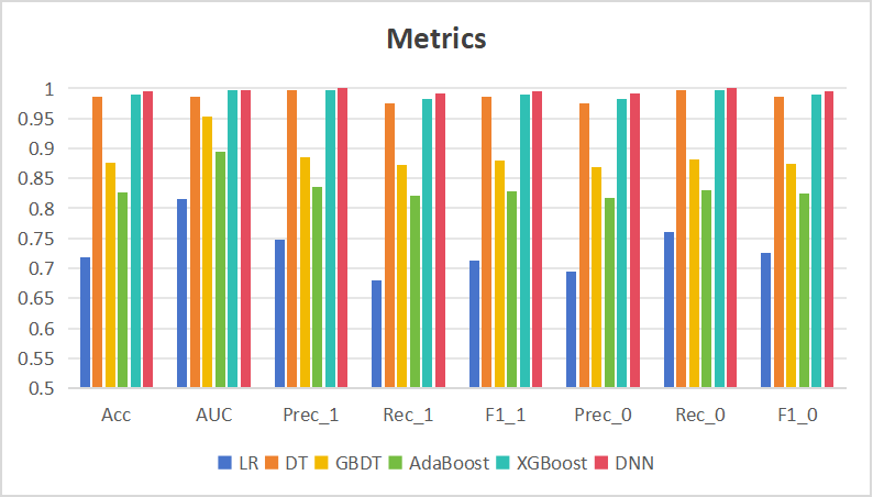
Figure 7. Comparison of model metrics.

4.4. Feature selecting assessment

In this section, the prediction of the dataset before feature selecting and the dataset after feature selecting was performed by DNN respectively, and the neural network was trained for the same 500 epochs with the same hyper-parameter settings, comparing the key metrics of the two. Table 3 recorded the comparative results of the two methods. The experimental results showed that the feature-selected dataset possesses better performance than the initial dataset in prediction, and Acc, AUC, Prec, Rec, and F1 are all higher than the initial model, which indicates that the feature selecting works well in this study.

Table 3. Feature selecting assessment

5. Discussion

The accuracy of DNN on the diabetes test set reached 99.5%, which possesses high accuracy. In this study, the structure of DNN was adjusted by adding several fully connected layers with a large number of neurons to ensure that the model learns the nonlinear relationship, and there was also a dropout layer to make sure that the model doesn't suffer from the problem of overfitting. As for the diagnosis of diabetes, the results had a very complex nonlinear relationship with the sample features, so the DNN in this paper can get better results.

There are some limitations in the present study. At first, the small number of features in the model does not guarantee reliability in clinical applications. Secondly, the dataset used needs to consider more types of samples.

6. Conclusion

In this study, a diabetes dataset was selected to be used for diabetes diagnosis research, and feature selecting was carried out by calculating the correlation coefficient, followed by applying SMOTE sampling to solve the data imbalance problem, and then training and prediction were carried out by deep neural network, and the final accuracy reached 99.5%, and the model metrics were compared with other machine learning models.

This study realized the diagnosis of diabetes by deep neural network and achieved certain research results, which makes the diagnosis of diabetes more convenient, and can effectively reduce the medical cost, improve the diagnostic efficiency, protect the patient's privacy, and safeguard the daily life. In the future, it is hoped that diabetes diagnosis can be realized through more and more specific features to improve the accuracy and credibility of diagnosis.

References

[1]. Wu F et al. 2023 Research on diabetes prediction model based on LightGBM model Chn. Health. Std. Man. 14 64-7
[2]. Zimmet et al. 2014 Diabetes: a 21st century challenge Lancet Diabetes Endocrinol. 2 56-64
[3]. Smith J W, Everhart J E, Dickson W C, Knowler W C and Johannes R S 1988 Using the ADAP learning algorithm to forecast the onset of diabetes mellitus In Proceedings of the Symposium on Computer Applications and Medical Care 261-5
[4]. Fernández et al. 2018 SMOTE for learning from imbalanced data: progress and challenges, marking the 15-year anniversary J. Art. Int. Res. 61 863-905
[5]. Myers, Leann and Maria J S 2004 Spearman Correlation Coefficients, Differences between. In Encyclopedia of Statistical Sciences (eds S. Kotz, C.B. Read, N. Balakrishnan, B. Vidakovic and N.L. Johnson)
[6]. LeCun Y, Bengio Y and Hinton G 2015 Deep learning Nature 521 436-44
[7]. LaValley and Michael P 2008 Logistic regression Circulation 117 2395-9
[8]. Song Y and L U Ying 2015 Decision tree methods: applications for classification and prediction Shanghai Arch. Psy. 2 130
[9]. Liang W et al. 2020 Predicting hard rock pillar stability using GBDT, XGBoost, and LightGBM algorithms Mathematics 8 765
[10]. Hastie T et al. 2009 Multi-class adaboost Stat. Inter. 2 349-60
Cite this article
Chen,Z. (2024). Development and validation of a deep learning-based model for diabetes diagnosis. Applied and Computational Engineering,76,317-325.
Data availability
The datasets used and/or analyzed during the current study will be available from the authors upon reasonable request.
Disclaimer/Publisher's Note
The statements, opinions and data contained in all publications are solely those of the individual author(s) and contributor(s) and not of EWA Publishing and/or the editor(s). EWA Publishing and/or the editor(s) disclaim responsibility for any injury to people or property resulting from any ideas, methods, instructions or products referred to in the content.
About volume
Volume title: Proceedings of the 2nd International Conference on Software Engineering and Machine Learning
© 2024 by the author(s). Licensee EWA Publishing, Oxford, UK. This article is an open access article distributed under the terms and
conditions of the Creative Commons Attribution (CC BY) license. Authors who
publish this series agree to the following terms:
1. Authors retain copyright and grant the series right of first publication with the work simultaneously licensed under a Creative Commons
Attribution License that allows others to share the work with an acknowledgment of the work's authorship and initial publication in this
series.
2. Authors are able to enter into separate, additional contractual arrangements for the non-exclusive distribution of the series's published
version of the work (e.g., post it to an institutional repository or publish it in a book), with an acknowledgment of its initial
publication in this series.
3. Authors are permitted and encouraged to post their work online (e.g., in institutional repositories or on their website) prior to and
during the submission process, as it can lead to productive exchanges, as well as earlier and greater citation of published work (See
Open access policy for details).