1. Introduction

As the society is filled of the data which recently keep proliferating. The machine learning represents a groundbreaking field at the intersection of the computer science and the artificial intelligence (AI) [1], where the primary goal is focusing on the algorithm and the model to make a better prediction, or even the decision. Thus, the machine learning has played a progressively role in human science since 20th century and it can execute the manual projects that transcend our abilities¹. Essentially, it gives the machine the ability to learn patterns or models, make the decision, and take the actions based on the data. Among the vast of the machine learning, there exists several specialized methods, such as supervised learning and unsupervised learning [2], where supervised learning is a subset of machine learning where algorithms are trained using labeled datasets to classify data or make predictions [1]. On the other hand, unsupervised learning involves using machine learning algorithms to analyze and cluster unlabeled datasets. They both includes varieties of algorithms which they each uniquely have their strengthens and characteristics. In this context, this paper is going to delve into three of these detailed methods which are the simple linear regression, the k-means clustering, and the decision tree, after that you will see what the differences are. Firstly, the simple linear regression is a technique used to find the relationship between independent variable and the dependent variable, modelling by a straight-line relationship, and it is used to analyze the labeled data which basically just add meaningful tags or labels or class to the observations [3]. For k-means clustering, it is an iterative algorithm that aims to divide a dataset of ‘n’ data points into ‘k’ clusters or groups [4], and the k-means clustering is used in the unlabeled data which is the opposite of the linear regression. Lastly, the decision tree is the non-parametric supervised learning algorithm, which is used for both classification and regression tasks [5].

2. Linear Regression

2.1. Algorithm

Linear regression is a supervised learning algorithm used for regression tasks. Its primary objective is to establish a linear relationship between a dependent variable (target) and one or more independent variables (features) [3]. The regression model describes the relationship variables by fitting in a line based on the data [6]. This equation can then be used for prediction and commonly the equation is

\( Y= {b_{0}}+ {b_{1}}x+ϵ \) (1)

, where the b_0 stands for the intersection of the line and Y-axis, and b_1 represents the slope of the line, and the error in the resultant prediction is donated by \( ε [7] \) . It is kind of the same as the linear formula, except the linear regression contains the error, because it is going to find the best prediction based on a brunch of data. When dealing with the linear regression model, there are several steps to be followed.

When working with a linear regression model, a systematic approach is crucial for achieving accurate and meaningful results. The first step in this process is obtaining the necessary data, ensuring it is comprehensive, clean, and well-structured. Subsequently, the exploration of the dataset is paramount, involving the calculation of descriptive statistics and the creation of visualizations to gain insights into the data's distribution and characteristics. Slicing the data, or selecting relevant features and target variables, comes next, a critical step in preparing for model creation. Building the linear regression model itself is the subsequent phase, where mathematical relationships between the variables are established. Finally, evaluating the model is imperative to assess its predictive performance, employing metrics like mean squared error or R-squared to quantify its accuracy and reliability. These sequential steps in linear regression modeling ensure a methodical and well-informed approach to data analysis and prediction [6]. Figure 1 will give you a better visualization, where it begins with data preparation, where raw data is organized into features and target variables. Feature extraction refines these features to enhance the model's ability to capture patterns. Next, a suitable machine learning model is selected and trained on the data. The model's performance is then assessed by comparing its predictions to the actual training data, using quality metrics to quantify its accuracy. This evaluation informs adjustments to the machine learning algorithm or pipeline, with the goal of improving the model's ability to generalize and make accurate predictions on new, unseen data [8].

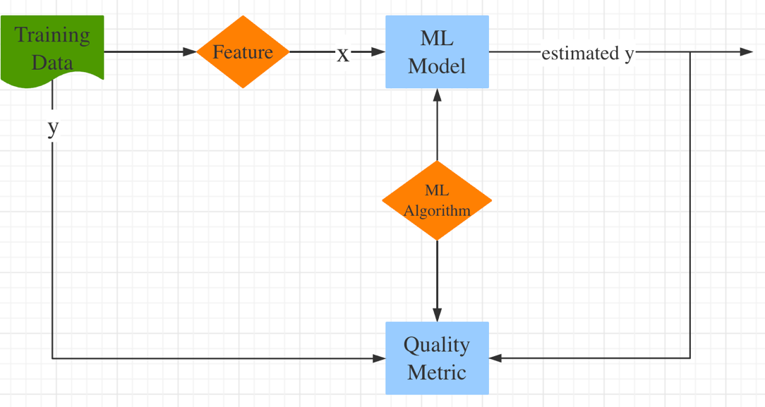
Figure 1. ML model

2.2. Application

Starting with a detailed example about linear regression by discussing the relationship of a person’s happiness comparing to his/her income to illustrate about the method. From the website of Bevans, Rebecca, it shows us a data set with 498 observations. In the dataset, it gives us a list of the value of the happiness and its corresponding income [9]. Then next thing to do is importing the data in your programming tools. Step 2 is crucial, as it involves verifying whether the data meets the assumptions of linear regression, such as linearity, independence of errors, and normality of residuals. Step 3 involves performing the linear regression analysis itself, estimating coefficients and assessing statistical significance. After regression analysis, Step 4 involves checking for homoscedasticity, which examines whether the variability of the residuals is constant across different levels of the independent variables. Lastly, in Step 5, the results can be visualized using various plots and graphs, such as scatterplots, fitted line plots, or residual plots, to help interpret the model and assess its goodness of fit. These steps collectively guide the process of using linear regression to gain insights and make predictions from data. In this example, it calculates the relationship or effect between the independent variable and the dependent variable, in this case is income and happiness, by using the lm() function which is linear model. Then you can use the summary function which will return a table, in the following image, of showing the minimum, maximum, the first quartiles, the residuals and so many other information to help you get the equation. Through these outcomes, it can build a regression equation by the given data set. What’s more, you can also check the p-value (2.2e-16 < 0.001) to indicate if the predicted model fits the data. Furthermore, you will finally find out there is a positive relationship between income and happiness with a slope 0.713, which means that for every unit increase in income, the value of the happiness will increase 0.713 as well.

Table 1. Summary of Residuals

Table 2. Summary of Coefficients

Table 3. Summary of residuals standard error

In addition to only represent the data table, it is also useful to use the graph to represent which will be easier to visualize. In the example, there is only one variable, thus it can be used a scatterplots graph to represent all the data and create a best-fit line to estimate the prediction by using geo_smooth() function, typing in lm method [9]. The figure 2 will show you the outcome figure with the estimated linear equation which has the best description of the predicted line.

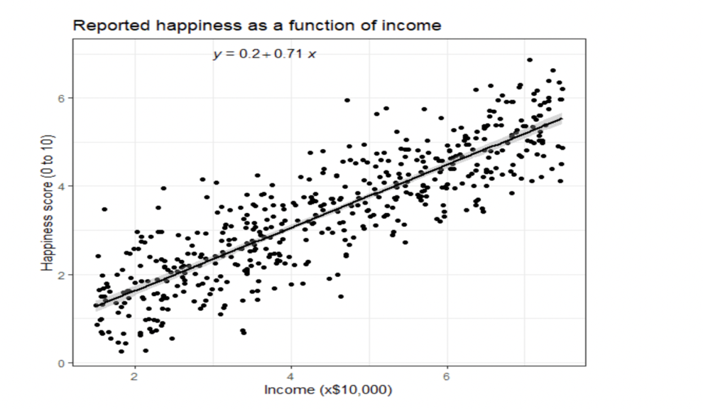
Figure 2. (the predicted line of the income and happiness score)

2.3. Cons and Pros

Linear regression offers several advantages, particularly excelling when data exhibits linear separability. Its simplicity makes it easy to implement, interpret, and train, making it accessible to a wide range of users. Furthermore, it can effectively mitigate overfitting through techniques like dimensionality reduction, regularization, and cross-validation. Additionally, one notable benefit is its capability for extrapolation, allowing it to make predictions beyond the scope of the training data. However, linear regression comes with its share of limitations. Its fundamental assumption of a linear relationship between dependent and independent variables can lead to suboptimal results when dealing with nonlinear data. It is also sensitive to noise and outliers, potentially impacting the model's accuracy. Moreover, multicollinearity, the presence of highly correlated independent variables, can pose challenges, causing instability in coefficient estimates and making it harder to interpret the individual effects of predictors. Careful consideration of these pros and cons is essential when deciding whether to use linear regression in a specific modeling task [7].

3. K-means

3.1. Algorithm

K-means is an unsupervised learning and used for the unlabeled data. Its primary goal is to find groups in the data where the groups are represented by the variable K [10]. Specifically, K-means is to partition a dataset into distinct groups, or clusters, based on the similarity of data points [11]. The algorithm begins by randomly selecting K initial cluster centers, where K represents the desired number of clusters. Then, it iteratively assigns each data point to the nearest cluster center and recalculates the centroids of these clusters. This process continues until convergence, where the cluster assignments no longer alter significantly, or a predetermined number of iterations is reached. In other words, K-means clustering is like organizing a collection of items into distinct groups. You start by deciding how many groups you want, which is the "K" in K-means. Then, the algorithm goes through each item and assigns it to one of these groups, making sure that each item belongs to exactly one group. The idea is to create groups where the items within each group are like each other and different from items in other groups. This way, you can uncover patterns or similarities in your data by organizing it into these non-overlapping clusters [11]. In this process, finding the center seems intuitively to find the average of all the points [12]. Thus, in algebraically, it can be expressed as equation (2).

\( {c_{k}}=\frac{1}{|{S_{k}}|}\sum _{pϵ{S_{k}}}{x_{p}} \) (2)

where \( {c_{k}} \) denotes as the centroid of the kth cluster, \( { x_{p}} \) used to group a set of P points, denoted as \( {x_{1}} \) , \( {x_{2}} \) , …, \( {x_{p}} \) , and \( {s_{k}} \) means all the points in each cluster, which those points belonging to kth cluster as equation (3) [12].

\( {S_{k}}=\lbrace p | if {x_{p}} belongs to the {k^{th}} cluster\rbrace \) (3)

Finally, when clustering the points into groups, it's obvious that each point should belong to the group whose center is closest to it. To put it in math terms for a specific point \( {x_{p}} \) , It can be said that this point should be part of the cluster where the distance between the point and the cluster's center (called centroid which is \( {∥{x_{p}}-{c_{k}}∥_{2}} \) ) is the smallest. In mathematically, the point \( {x_{p}} \) belongs to or cluster k if it satisfied the equation (4) [12].

\( {a_{p}}=\underset{k=1,...,k}{argmin}{{∥{x_{p}}-{c_{k}}∥_{2}}} \) (4)

3.2. Application

In K-means model, it is easy and obviously to understand the process by showing the graph. In Figure 3, Step 1 gives you the distribution of the data, representing by the points. Then it will be grouping into several clusters randomly, which the colored dots are very scattered in the Step 2. Also, it will be setting the centroid randomly where they are shown in several big circles in Figure 5. Then the next step is going to calculate or measure the distance between each centroid and all the points, which there are many methods to achieve that, such as the Euclidean Distance, the Cos Similarity, and the Manhattan Distance where the Euclidean Distance, shown in the equation (5), is a measure of straight-line distance between two points in space by using the Pythagorean Theorem,

\( d=\sqrt[]{{({x_{2}}-{x_{1}})^{2}}+{({y_{2}}-{y_{1}})^{2}}} \) (5)

the Euclidean Distance is a metric used to measure the similarity between two vectors by calculating the cosine of the angle between them [13], and the Manhattan Distance is measured the two points along the axes at the right angles [14]. After calculating the distances, you will know the distances of the data points to each centroid and you can group these points, in this case filling the same color as the centroids and Step 4 will show you how will the points be distributed. Furthermore, you can re-center the previous centroids to the new central place, or the average of the grouping points which is shown on the Step 5. It might not be able to cluster assignments no longer alter significantly at the first iteration. Rather than that, you should keep iterating until the centroid never change. Then Step 6 provides the results.

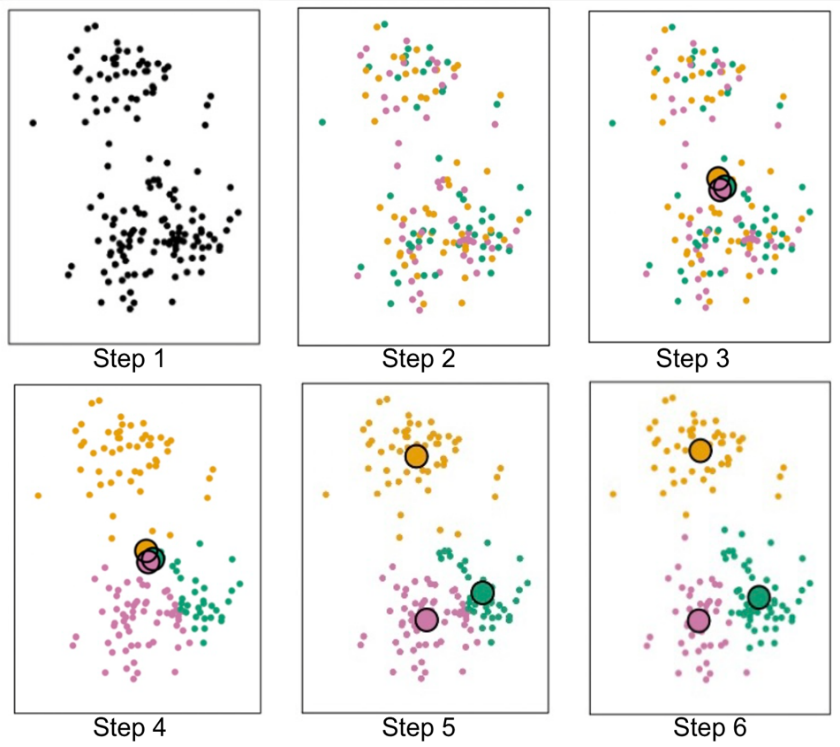
Figure 3. process of Decision Tree method

3.3. Cons and Pros

K-means clustering offers several advantages. Firstly, it exhibits high performance, being computationally efficient and capable of handling large datasets. Secondly, it's easy to use and understand, making it accessible to users with various levels of expertise. Thirdly, it can be applied to unlabeled data, allowing for data exploration and insight discovery. Finally, K-means results are relatively straightforward to interpret, as clusters are well-defined. However, there are drawbacks to consider. K-means can be sensitive to initializations, leading to varying results in different runs. It also assumes that clusters are spherical in shape, which may not be appropriate for all datasets. Additionally, the method requires users to manually specify the number of clusters (K), which can be challenging without prior knowledge. Lastly, K-means tends to create clusters even when the data may not naturally exhibit distinct groupings, potentially leading to over-segmentation [15].

4. Decision Tree

4.1. Algorithm

A decision tree is a popular machine learning algorithm used for both classification and regression tasks. In Figure 4, a decision tree is a tree-like structure which consists of several key components. At its outset is the root node, which represents the entire dataset and subsequently branches into two or more homogeneous subsets during the splitting process. These divisions occur at decision nodes, where the tree makes choices based on specific criteria or features. At the terminus of each branch lie the leaf or terminal nodes, signifying final outcomes or classifications. To optimize the tree's efficiency and prevent overfitting, the process of pruning is employed, removing sub-nodes and simplifying the structure. Together, these components create a hierarchical structure, with branches and sub-trees representing different sections of the overall decision-making process, and nodes forming parent-child relationships as they divide and inherit attributes [16].

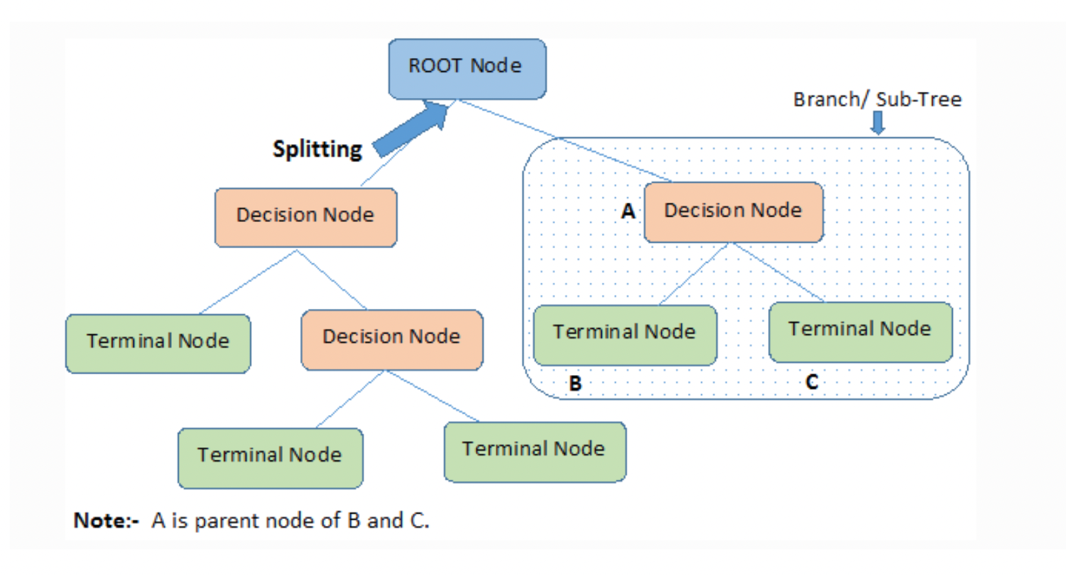
Figure 4. A basic structure of a Decision Tree [16]

In a decision tree, each node acts like a question about a specific characteristic or feature of the data. When you answer the question, you follow an edge to the next node, which asks another question based on your answer. This process keeps repeating, forming a tree-like structure, until you reach a final answer or outcome at the end of a branch. It's like a series of yes-or-no questions that guide you to a conclusion step by step.

4.2. Application

To have a better understanding about the process of the Decision Tree. Table 4 shows you the data we are using for next and there are 6 Safe loans and 3 Risky which is the predicted response. The term column represents the number of years that the person needs to pay the loan and the credit means their credit history.

Table 4. The Data

The next step is going to check whether the data is satisfied the certain decision node which is “Credit?” in Figure 5, then it will, in this case, split to 3 tracks which tells us if the person’s credit is either excellent or fair or poor and, in the figure, two individuals, both initially possessing excellent credit, continue to maintain a safe loan status as predicted. Meanwhile, three individuals with an existing excellent credit history are projected to maintain a safe loan status. Also, there is a people have a fair credit will have a safe load status. One individual, initially categorized as having fair credit, is anticipated to transition to risky loan status. Lastly, three individuals already possessing poor credit are expected to retain their predicted risky loan status. In figure 6, By factoring in the "term" parameter, one can effectively evaluate the credit statuses of individuals based on their chosen loan durations. Among the four individuals who have selected a 3-year loan term, a majority are expected to maintain a safe loan status, while two individual is predicted to fall under a risky loan status. Conversely, among the three individuals who have committed to a 5-year loan term, one group is projected to have a safe loan status (1 person), while the other group is foreseen to carry a risky loan status (2 people). This refined perspective offers a more comprehensive insight into the credit dynamics of individuals based on their individual loan terms.

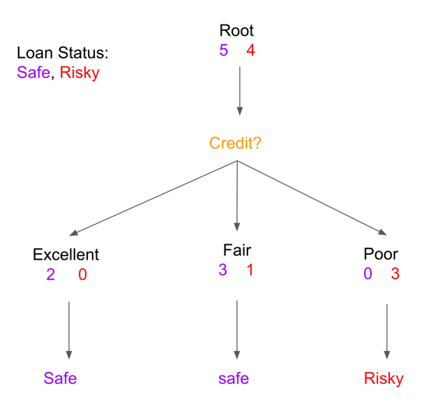
Figure 5. filtering by the parameter Credit

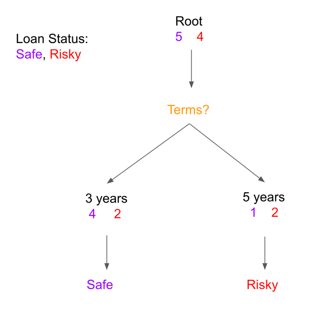
Figure 6. filtering by the parameter Terms

During this process, you can check the error of each parameter or how good will be the parameter using in the model by taking the mistakes, in this case is the person’s past loan status is not the same as his/her predicted status, divided by the total number, for instance for the Figure 10, there are 1 (0 + 1 + 0) mistakes, and the total number is 9, thus the error will be 1 over 9 which is approximately 0.11. The same idea for the Figure 11, the error will be 3 over 9 which will be approximately 0.33. Next, by comparing the error, it can tell that using the parameter credit will be the winner. In this example, even though it is not that complicated, at least you might have a basic idea about what is the decision tree and how it works usually.

4.3. Pros and Cons

Decision trees offer several advantages in machine learning. They provide a straightforward, visual representation of decision-making processes and excel at capturing non-linear patterns in data. Moreover, they prove useful in predicting missing values and are compatible with feature engineering techniques. However, it's crucial to be mindful of potential disadvantages, such as the risk of overfitting and the sensitivity of decision trees to small variations in input data. To mitigate these concerns, balancing the dataset before model training is often necessary for optimal results [17].

5. Conclusion

This paper delved into three fundamental machine learning techniques: linear regression, k-means clustering, and decision trees. These methods were applied to a dataset, leading to the identification of insightful patterns and insights. The findings emphasized the strengths and limitations of each technique. Linear regression effectively modeled relationships between variables, k-means clustering proved useful for data point grouping, and decision trees offered interpretability and decision-making abilities. These techniques possess broad applications across various fields, with their effectiveness depending on the specific problem and dataset. This study contributes to an enhanced understanding of these techniques and their potential for data analysis and prediction. Future research opportunities include exploring advanced variations of these methods and their application in real-world contexts. In summary, linear regression, k-means clustering, and decision trees retain their significance as essential tools in the realm of data analysis, offering valuable insights and predictive capabilities.

References

[1]. “What Is Machine Learning?” IBM, www.ibm.com/topics/machine-learning. Accessed 21 Sept. 2023.
[2]. Tucci, Linda, and Ed Burns. “What Is Machine Learning and How Does It Work? In-Depth Guide.” Enterprise AI, TechTarget, 15 Sept. 2023, www.techtarget.com/searchenterpriseai/definition/machine-learning-ML.
[3]. K, H., Khanra, S., Rodriguez, R. V., & Jaramillo, J. (2022). Machine Learning for Business Analytics : Real-Time Data Analysis for Decision-Making. Productivity Press. https://doi.org/10.4324/9781003206316
[4]. bernie2436bernie2436 22.9k4949 gold badges151151 silver badges244244 bronze badges, et al. “What Is the Difference between Labeled and Unlabeled Data?” Stack Overflow, 1 Feb. 1960, stackoverflow.com/questions/19170603/what-is-the-difference-between-labeled-and-unlabeled-data.
[5]. “What Is a Decision Tree.” IBM, www.ibm.com/topics/decision-trees. Accessed 8 Oct. 2023.
[6]. “What Is Deep Learning?” IBM, www.ibm.com/topics/deep-learning. Accessed 22 Sept. 2023.
[7]. “Linear Regression for Machine Learning: Intro to ML Algorithms.” Edureka, 2 Aug. 2023, www.edureka.co/blog/linear-regression-for-machine-learning/#advantages.
[8]. “What Is a Machine Learning Pipeline?” What Is a Machine Learning Pipeline?, valohai.com/machine-learning-pipeline/. Accessed 7 Oct. 2023.
[9]. Bevans, Rebecca. “Simple Linear Regression: An Easy Introduction & Examples.” Scribbr, 22 June 2023, www.scribbr.com/statistics/simple-linear-regression/.
[10]. Trevino, Andrea. “Introduction to K-Means Clustering.” Oracle Blogs, blogs.oracle.com/ai-and-datascience/post/introduction-to-k-means-clustering. Accessed 7 Oct. 2023.
[11]. James, Gareth, et al. An Introduction to Statistical Learning: With Applications in R. Springer, 2022.
[12]. 8.5 K-Means Clustering - Github Pages, jermwatt.github.io/machine_learning_refined/notes/8_Linear_unsupervised_learning/8_5_Kmeans.html. Accessed 8 Oct. 2023.
[13]. Author: Fatih Karabiber Ph.D. in Computer Engineering, et al. “Cosine Similarity.” Learn Data Science - Tutorials, Books, Courses, and More, www.learndatasci.com/glossary/cosine-similarity/. Accessed 8 Oct. 2023.
[14]. Manhattan Distance, xlinux.nist.gov/dads/HTML/manhattanDistance.html. Accessed 8 Oct. 2023.
[15]. “K-Means Pros & Cons.” HolyPython.Com, 25 Mar. 2023, holypython.com/k-means/k-means-pros-cons/.
[16]. “Decision Tree Algorithm, Explained.” KDnuggets, www.kdnuggets.com/2020/01/decision-tree-algorithm-explained.html. Accessed 9 Oct. 2023.
[17]. Team, Towards AI. “Decision Trees Explained with a Practical Example.” Towards AI, 6 Jan. 2023, towardsai.net/p/programming/decision-trees-explained-with-a-practical-example-fe47872d3b53.
Cite this article
Huang,X. (2024). Predictive Models: Regression, Decision Trees, and Clustering. Applied and Computational Engineering,79,124-133.
Data availability
The datasets used and/or analyzed during the current study will be available from the authors upon reasonable request.
Disclaimer/Publisher's Note
The statements, opinions and data contained in all publications are solely those of the individual author(s) and contributor(s) and not of EWA Publishing and/or the editor(s). EWA Publishing and/or the editor(s) disclaim responsibility for any injury to people or property resulting from any ideas, methods, instructions or products referred to in the content.
About volume
Volume title: Proceedings of the 4th International Conference on Signal Processing and Machine Learning
© 2024 by the author(s). Licensee EWA Publishing, Oxford, UK. This article is an open access article distributed under the terms and
conditions of the Creative Commons Attribution (CC BY) license. Authors who
publish this series agree to the following terms:
1. Authors retain copyright and grant the series right of first publication with the work simultaneously licensed under a Creative Commons
Attribution License that allows others to share the work with an acknowledgment of the work's authorship and initial publication in this
series.
2. Authors are able to enter into separate, additional contractual arrangements for the non-exclusive distribution of the series's published
version of the work (e.g., post it to an institutional repository or publish it in a book), with an acknowledgment of its initial
publication in this series.
3. Authors are permitted and encouraged to post their work online (e.g., in institutional repositories or on their website) prior to and
during the submission process, as it can lead to productive exchanges, as well as earlier and greater citation of published work (See
Open access policy for details).