1. Introduction

Predicting stock prices is a crucial aspect of financial markets. Precise forecasting of stock prices can lead to financial gains and informed decision-making. However, the increase in global political conflicts, wars, and terrorist activities has resulted in heightened instability in stock prices. Therefore, it is important to evaluate the accuracy of forecasting when applying different algorithms.

Autoregressive Integrated Moving Average (ARIMA) Model is a traditional mathematics approach to predict time series. The autoregressive (AR) model was first introduced by Yule in 1926. The basic idea is to express the current value of a time series as a linear combination of its previous values. The moving average (MA) model was proposed by Slutzky in 1937 to enhance time series data by calculating the weighted average of past observations. Autoregressive Moving Average (ARMA) model was proposed by Box and Jenkins in 1970 [1]. The ARMA model was created by merging the advantages of both models.

Recurrent Neural Networks (RNNs) were developed in the 1980s to process sequential data by preserving a state that captures information from previous time steps [2]. Nevertheless, RNNs faced challenges in efficiently acquiring knowledge of long-term connections because of the occurrence of vanishing and exploding gradient issues, which ultimately restricted their effectiveness. In 1997, Sepp Hochreiter and Jürgen Schmidhuber pioneered the Long Short-Term Memory (LSTM) [3]. The LSTM was designed to address the limitations of standard RNN by introducing a memory cell capable of maintaining its internal state over long periods.

During the late 2000s to early 2010s, the advancement of computing power allowed deep learning to effectively handle nonlinearity and complexity in time series forecasting [4]. Researchers began applying LSTM in the fields of economics and finance. This includes using LSTM for tasks like time series forecasting and predicting the volatility of the S&P100 [5-6]. In 2018, T Fischer and C Krauss applied LSTM to analyze the performance of the S&P500 from December 1992 to October 2015 [7]. The researchers discovered that the LSTM algorithm surpasses memory-free classification techniques, such as random forest, deep neural net, and logistic regression classifier, in terms of performance.

This paper presents an introduction to the LSTM algorithm and conducts a performance comparison with the ARIMA model. The selection of ARIMA is based on its status as a well-known traditional mathematical method and its capability to handle non-stationary data.

The code for the LSTM algorithm is implemented using the early-stopping method. This paper also compares the performance of LSTM and ARIMA in S&P500 stock prediction. To evaluate the performance of LSTM algorithm in different stocks, the author selects 6 typical US stocks and applies the optimized LSTM algorithm. This research illustrates the use of deep learning algorithms to optimize the forecast of stock price. Furthermore, this paper shows a negative correlation between stock volatility and accuracy. Researchers can use the results of this paper to further improve and optimize the LSTM models.

2. ARIMA

The ARMA model is employed to analyze individual time series data by merging the Autoregressive (AR) and Moving Average (MA) models. The ARIMA model, a variant of ARMA, includes differencing to address non-stationary data. The ARIMA (p,d,q) model consists of three essential elements.

The initial model is AR, often known as Autoregression (p). This component represents the correlation between a current observation and a previous observation.

It assumes that the current value of the series can be explained by a linear combination of its previous values, which can be written as

\( {Y_{t}}=\sum _{i=1}^{p}{ϕ_{i}}{Y_{t-i}}+{ϵ_{t}}\ \ \ (1) \)

where \( {Y_{t}} \) represents the value of time series at time \( t \) , \( {ϕ_{i}} \) are the auto-correlation coefficients. Each \( {ϕ_{i}} \) represents the influence of the time series \( i \) periods ago at current value \( {Y_{t}} \) . \( {Y_{t-i}}  \) elaborates the value of time series at time \( t-i \) , where \( i \) range from \( 1 \) to \( p \) . \( {ϵ_{t}} \) are random values at time \( t \) .

The second component is I, also known as the Integrated part (d). To make the time series stationary, measuring the differences in observations at various times is necessary. To be more specific, if the original time series is stationary, then \( d=0 \) . However, if not stable, the difference is performed, and the Augmented Dickey-Fuller (ADF) that is used to test the time series is stable. In general, the number of differences does not exceed 2 times. This part can be written as

\( Y_{t}^{ \prime }={Y_{t}}-{Y_{t-1}}\ \ \ （2） \)

The last component is MA, commonly referred to as the Moving Average (q), which captures the relationship between an observation and a residual error from a moving average model applied to lagged observations, which can be illustrated as

\( {Y_{t}}=μ+{ϵ_{t}}+\sum _{i=1}^{q}{θ_{i}}{ϵ_{t-i}}\ \ \ （3） \)

In this equation, \( μ \) is consistent, \( {ϵ_{t}} \) is a random error term at the current time point, \( {ϵ_{t-i}} \) is error term for the previous point in time, \( {θ_{i}} \) is the coefficient of the MA component.

By summing these three models, a composite ARIMA model of order \( (p,d,q) \) can be created. The forecast model employed in this experience is an ARIMA (6, 1, 1) model, which serves as the basis for modeling the forecast. While this model may not be the most efficient, it serves as a valuable starting point for building a model, as demonstrated by the explanatory experiments [8].

3. LSTM

Long Short-Term Memory (LSTM) is a type of Recurrent Neural Network (RNN). Different from traditional RNN, LSTM introduces the memory cell, which can capture and retain long-term dependencies in previous data. Before introducing LSTM, Recurrent Neural Network (RNN) will be introduced first.

3.1. RNN

The traditional RNN consists of three layers, including an input layer, a hidden layer, and an output layer. The input layer and output layer are used to input data and output data respectively.

The crucial component is the hidden layer, which contains several nodes. The nodes of the hidden layer are connected to each other through links called "synapses". Every synapse in the neural network is assigned a weight that corresponds to each node in the input layer. These weights serve as arbiters, determining which signals or inputs are permitted to pass through. Moreover, the weights indicate the influence exerted on the hidden layer. However, when dealing with long sequences, RNNs often face gradient vanishing or exploding problems when processing long sequences referring to Figure 1.

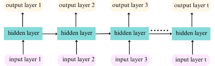
Figure 1. The principle of traditional RNN

3.2. LSTM

LSTM is specifically made to overcome the long-term dependency issue. The main difference between LSTM and RNN is that an LSTM unit captures three key components known as gates. These gates include the Forget gate, the Input gate, and the Output gate. The Forget gate determines which information should be forgotten, the Input gate quantifies the importance of the new information and decides what new information should be stored, and the Output gate controls what kind of information is to be output [4]. Refer to the following image.

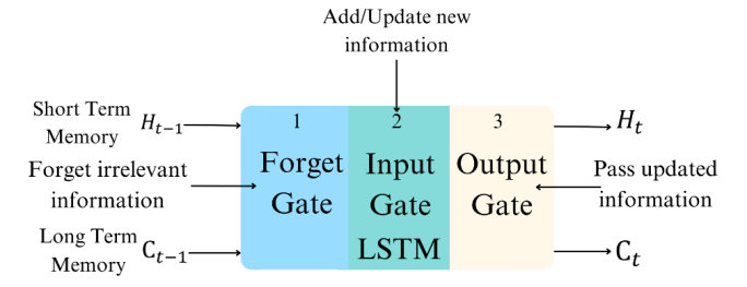
Figure 2. The principle of LSTM

The LSTM core code is as follows:

# Constructing LSTM model

model = Sequential()

model.add(LSTM(128, return_sequences=True, input_shape=(x_train.shape[1], 1)))

model.add(LSTM(64, return_sequences=False))

model.add(Dense(25))

model.add(Dense(1))

# Compilation model

model.compile(optimizer='adam', loss='mean_squared_error')

# train model

early_stopping = EarlyStopping(monitor='val_loss', patience=10, restore_best_weights=True)

history = model.fit(x_train, y_train, batch_size=1, epochs=20, validation_split=0.2, callbacks=[early_stopping])

The Constructing LSTM model consists of two LSTM layers followed by two dense layers. The LSTM layers are designed to capture temporal dependencies in the input sequence data, while the dense layers are used for transforming the learned features into the final prediction.

In the Compilation model part, “adam” and “mean squared error” are applied to be the optimization algorithm and the loss function.

In the train model part, early stopping is used to stop overfitting. It monitors the performance of the model on validation losses. If the validation loss does not improve, the training process will stop.

4. Experience

4.1. Dataset

The first experience is the comparison of LSTM and ARIMA.

The author collected S&P500 index(^GSPC) historical daily stock prices from 2022, May 01 to 2024, May 01 on the Yahoo Finance Website [9]. The “Close” variable is selected as the feature input into both the ARIMA and LSTM models. In ARIMA, 70% of the data was used to train, and 30% of it was used to test. In LSTM, 56% of the data was used to train, 14% of it was used to validate, and 30% of it was used to test. In the experimental figures, training data and validation data are simplified as “Train”, both in the first and second experiences.

The second experience is the performance of LSTM in different stocks.

The author collected S&P500 index(^GSPC), NASDAQ index(^IXIC), Apple index(AAPL), Google index(GOOGL), Meta index(META) and Nvidia index(NVDA) historical daily stock prices from 2022, May 01 to 2024, May 01 in the Yahoo Finance Website [9]. The “Close” variable was chosen as the feature input into LSTM models.

4.2. Evaluation metrics

In the first experience, the Root-Mean-Square Error (RMSE) is applied to calculate the reliability of forecast by a model. The RMSE equation is

\( RMSE=\sqrt[]{\frac{1}{n}\sum _{i=1}^{n}{({x_{i}}-x_{i}^{ \prime })^{2}}}\ \ \ （4） \)

where \( n \) is the whole quantity of measurements, \( {x_{i}} \) the real price, and \( x{ \prime _{i}} \) the predicted price.

In the second experience, the Relative RMSE is used to evaluate the accuracy of a prediction by a model. Compared with RMSE, Relative RMSE allows for a fair comparison of model performance across different stock data. Smaller values indicate lower model errors and better performance. The Relative RMSE equation is

\( Relative RMSE=\frac{RMSE}{\bar{y}}\ \ \ （5） \)

where \( \bar{y} \) is mean of actual values.

The Historical Volatility of Stocks is used to evaluate the volatility of different stocks, whose equations are as follows:

The Daily Percentage Returns can be calculated by

\( {R_{t}}=\frac{{P_{t}}}{{P_{t-1}}}-1\ \ \ （6） \)

where \( {R_{t}} \) is return on day \( t \) , \( {P_{t}} \) is close price on day \( t \) and \( {P_{t-1}} \) is close price on day \( t-1 \) ;

The standard Deviation of Daily Returns can be calculated by

\( σ=\sqrt[]{\frac{1}{N-1}\sum _{t=1}^{N}{({R_{t}}-\bar{R})^{2}}}\ \ \ (7) \)

where \( σ \) is standard deviation, \( \bar{R} \) is the mean of the daily returns.

Assuming 252 trading days happen during a year, the annualized volatility is

\( {σ_{annual}}=σ×\sqrt[]{252}\ \ \ (8) \)

4.3. Experimental Result

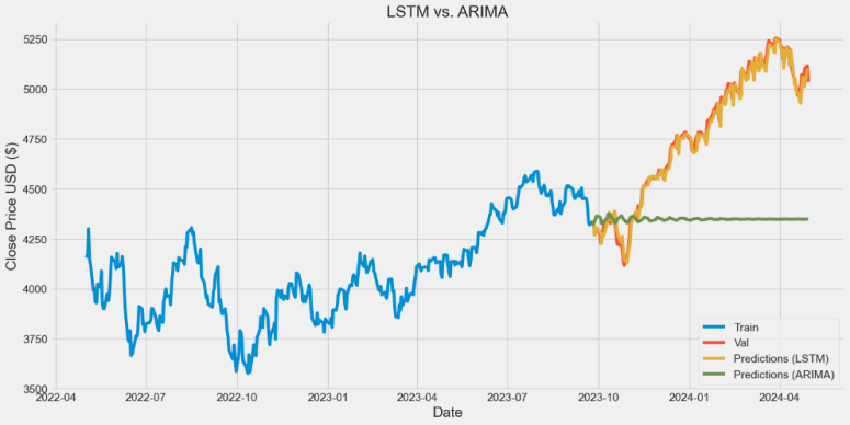
Figure 3. the result of LSTM vs. ARIMA

Table 1. the RMSE of LSTM and ARIMA

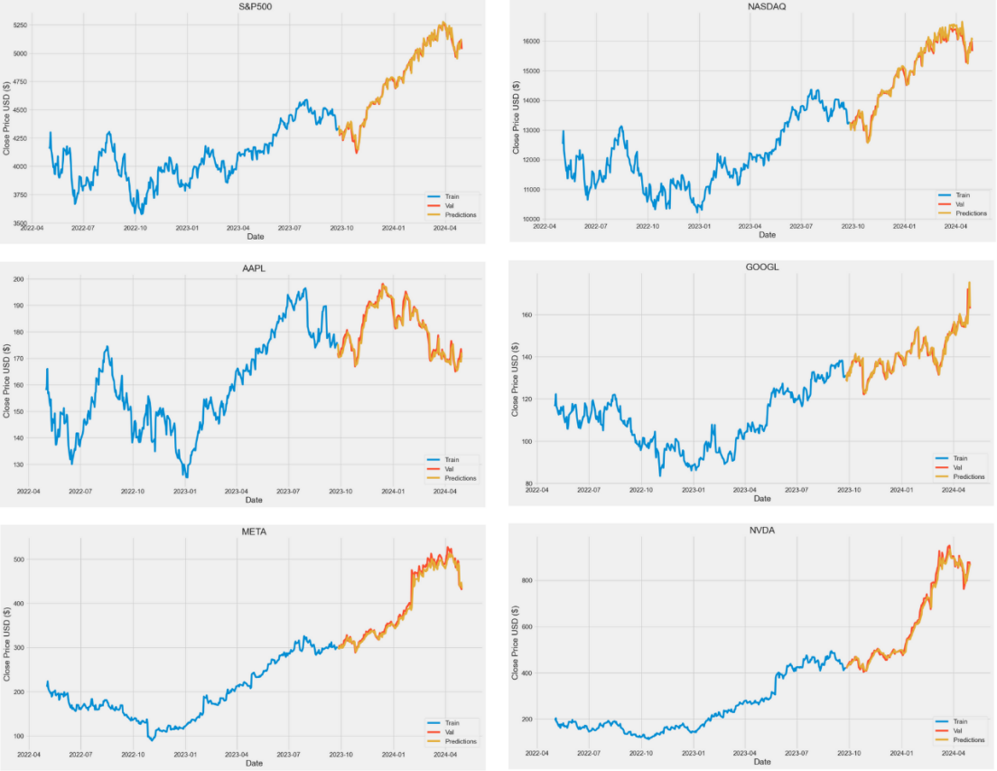
Figure 4. the result of LSTM prediction in different stocks

Table 2. The RMSE, Relative RMSE and Volatility in different stocks

For the first experience, the results are reported in Figure 3 and Table 1. The RMSE of LSTM and ARIMA are 39.702 and 533.812, respectively, resulting in a reduction in error rates of 92.563% achieved by LSTM. The RMSE figures demonstrate that LSTM models surpass ARIMA models by a substantial difference.

For the second experience, the outcomes are reported in Figure 4 and Table 2. In Table 2, the author sorted the data in ascending order using “Volatility” as the keyword. According to the experimental data, because the single stock price easily influences the RMSE, the Relative RMSE is more suitable as an evaluation indicator of prediction. Relative RMSE enables direct comparison of errors across datasets. The data indicate a generally positive correlation between volatility and Relative RMSE. As stock volatility increases, the Relative RMSE also rises, leading to a decrease in the accuracy of the LSTM algorithm.

5. Conclusion

With the development of machine learning, especially deep learning. the methods mentioned in this paper are gaining popularity among researchers in several areas. The important question pertains to the level of accuracy and efficacy exhibited by these new approaches in comparison to conventional approaches. The study examines the reliability of ARIMA and LSTM, two widely recognized algorithms for forecasting S&P500 stock prices. The findings suggest that the LSTM model outperforms the ARIMA model. The LSTM algorithm significantly enhances prediction accuracy, with a 92% improvement over ARIMA. Furthermore, this paper applies the LSTM algorithm to different stocks. The results indicate a negative correlation between the stock’s volatility and the accuracy of the LSTM algorithm. This paper exhibits certain limitations, for example, it only applies to S&P500 and 6 typical U.S. tech stocks, which results in a lack of verification using broader market and international data.

The main contribution of this paper is to highlight the advantages of using deep learning algorithms to analyse stock prices. It suggests that deep learning has the potential to be used in a wide range of prediction problems in the field of finance and economics. This paper explores the relationship between volatility and relative RMSE through the utilization of the LSTM algorithm. Researchers can decide the suitability of using LSTM by measuring volatility, thereby optimizing computational resources and time.

References

[1]. Box, George; Jenkins, Gwilym (1970). Time Series Analysis: Forecasting and Control. San Francisco: Holden-Day.
[2]. Medsker, L. R., & Jain, L. (2001). Recurrent neural networks. Design and Applications, 5(64-67), 2.
[3]. Hochreiter, S., & Schmidhuber, J. (1997). Long short-term memory. Neural computation, 9(8), 1735-1780.
[4]. Gers, F. A., Schmidhuber, J., & Cummins, F. (2000). Learning to forget: Continual prediction with LSTM. Neural computation, 12(10), 2451-2471.
[5]. Sagheer, A., & Kotb, M. (2019). Time series forecasting of petroleum production using deep LSTM recurrent networks. Neurocomputing, 323, 203-213.
[6]. Huck, N. (2009). Pairs selection and outranking: An application to the S&P 100 index. European Journal of Operational Research, 196(2), 819-825.
[7]. Fischer, T., & Krauss, C. (2018). Deep learning with long short-term memory networks for financial market predictions. European journal of operational research, 270(2), 654-669.
[8]. Ariyo, A. A., Adewumi, A. O., & Ayo, C. K. (2014, March). Stock price prediction using the ARIMA model. In 2014 UKSim-AMSS 16th international conference on computer modelling and simulation (pp. 106-112). IEEE.
[9]. Yahoo Finance. https://finance.yahoo.com
Cite this article
Wang,Z. (2024). Stock price prediction using LSTM neural networks: Techniques and applications. Applied and Computational Engineering,86,275-281.
Data availability
The datasets used and/or analyzed during the current study will be available from the authors upon reasonable request.
Disclaimer/Publisher's Note
The statements, opinions and data contained in all publications are solely those of the individual author(s) and contributor(s) and not of EWA Publishing and/or the editor(s). EWA Publishing and/or the editor(s) disclaim responsibility for any injury to people or property resulting from any ideas, methods, instructions or products referred to in the content.
About volume
Volume title: Proceedings of the 6th International Conference on Computing and Data Science
© 2024 by the author(s). Licensee EWA Publishing, Oxford, UK. This article is an open access article distributed under the terms and
conditions of the Creative Commons Attribution (CC BY) license. Authors who
publish this series agree to the following terms:
1. Authors retain copyright and grant the series right of first publication with the work simultaneously licensed under a Creative Commons
Attribution License that allows others to share the work with an acknowledgment of the work's authorship and initial publication in this
series.
2. Authors are able to enter into separate, additional contractual arrangements for the non-exclusive distribution of the series's published
version of the work (e.g., post it to an institutional repository or publish it in a book), with an acknowledgment of its initial
publication in this series.
3. Authors are permitted and encouraged to post their work online (e.g., in institutional repositories or on their website) prior to and
during the submission process, as it can lead to productive exchanges, as well as earlier and greater citation of published work (See
Open access policy for details).